Do All RF Radar Systems Need Their Own Transmitter?

No. Active radar uses a dedicated transmitter, which may be separate from the receiver. Passive radar detects objects using reflections of transmissions from other sources, such as radio or television broadcasts. It does not generate its own illuminating waveform, so its operation depends on the available external signals.

Can Radar Signal Processing Compensate for RF Hardware Limitations?

Partly. Processing can improve detection by integrating repeated echoes and correcting characterized amplitude, phase, or timing errors. Integration can reveal signals below the noise floor of an individual observation. However, processing cannot reliably restore information lost through clipping, severe distortion, or analog filtering, so the RF hardware must preserve the information needed for detection.

Can a Radar RF Cable Be Replaced Without Recalibrating the Channel?

Yes, if the approved replacement procedure permits it and verification confirms that the channel still meets its requirements. A replacement can change loss, delay, and phase despite matching the original cable’s length and connectors. The procedure and test results determine whether recalibration is needed and how much of the system it must cover.

How Do Radar and Electronic Warfare Systems Differ?

Radar detects objects and measures their position or motion through radio echoes. Electronic warfare (EW) encompasses electronic support, attack, and protection: gathering information from emissions, disrupting an opponent’s use of the spectrum, and protecting friendly systems. Both can use similar RF hardware and share integration concerns such as isolation, signal integrity, timing, and calibration.

RF Radar Systems: Signal Chain and Design Trade-offs

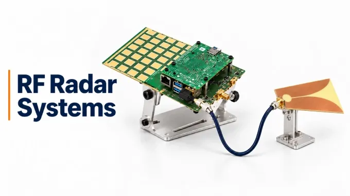
Active RF radar systems transmit a known waveform and analyze returning echoes to measure range, motion, and direction. Their RF hardware must deliver enough transmit energy while preserving much weaker echoes. Loss, noise, distortion, and transmitter leakage therefore constrain the usable performance of the complete signal chain.

How Does the RF Signal Chain in a Radar System Work?

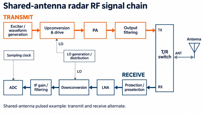
The RF signal chain prepares the waveform for transmission and conditions returning echoes for an analog-to-digital converter (ADC). In a shared-antenna pulsed radar, the transmit chain drives the antenna during each pulse, and the receiver captures echoes between pulses.

The radar RF front end includes the antenna-facing transmit and receive electronics. Local oscillator (LO) signals support frequency conversion, while frequency references and synchronized timing coordinate waveform generation and sampling for coherent operation.

Transmit Chain: Generating and Delivering the Required RF Waveform

The transmit chain raises the exciter’s low-power signal to the required antenna power while controlling unwanted spectral content.

Stage	Components and function
Waveform generation	The exciter creates the waveform. When a DAC is used, a reconstruction filter suppresses unwanted sampling images.
Conversion and drive	Frequency conversion, where required, establishes the RF band. Filters reject unwanted conversion products, and a driver amplifier supplies the power amplifier (PA’s) required input level.
Power amplification	The radar power amplifier raises the signal to the required RF output power.
Output filtering and monitoring	An output filter, where required, suppresses harmonics. Directional couplers supply samples to detectors that monitor forward or reflected power.

Three relationships govern the design:

Waveform fidelity: Some constant-envelope signals permit PA operation near saturation. Signals with varying amplitude may require output backoff to limit distortion.
Peak power and heat: Peak power determines instantaneous electrical stress. For rectangular pulses, average RF output equals peak power multiplied by duty cycle. Cooling must account for the amplifier’s efficiency and bias consumption under the intended operating conditions.
Power delivered to the antenna: The PA’s output rating does not establish the power at the antenna feed. A combined 3 dB loss through output filters, routing devices, and interconnects leaves approximately half the PA’s output power at the antenna.

Receive Chain: Protecting and Conditioning Weak Echoes

The receive chain must preserve weak-signal information while preventing strong inputs from damaging or overloading sensitive stages.

Antenna routing comes first. With a shared antenna, a T/R switch changes its connection between the transmit and receive paths. A circulator routes power between successive ports in a fixed direction. Separate antennas simplify this routing, but transmitter energy can still couple into the receiver.

The remaining functions are distributed through the receive path according to the architecture:

Function	Components and purpose
Input protection	A limiter restricts residual or unexpected RF power before it reaches sensitive components.
RF preselection	A filter attenuates signals outside the intended receive band.
Low-noise amplification	The LNA raises weak echoes while adding relatively little noise.
Frequency conversion, where required	A mixer uses an LO to translate received RF signals to an intermediate frequency (IF) for further amplification, filtering, and digitization.
ADC interfacing	An antialias filter constrains the ADC’s input spectrum. A driver, where needed, provides the required signal swing, impedance interface, and common-mode level.

Placement creates a trade-off. Preselection before the LNA reduces exposure to out-of-band interference, but its insertion loss also affects sensitivity. Protection requirements, interference levels, and available signal headroom determine the appropriate arrangement; one component order does not suit every radar.

Frequency Conversion, LO (Local Oscillator) Distribution, and Timing

These supporting paths establish conversion frequencies, sampling instants, and coordinated operation across the radar.

LO generation and distribution: Oscillators and synthesizers produce LO signals. Buffers and power dividers distribute them at the drive levels required by the mixers.
Frequency conversion: A mixer produces sum-and-difference frequency components, and filtering selects the required output. Conversion gain or loss affects the downstream signal level, while finite port isolation permits unwanted leakage.
Sampling clock: The clock determines when the ADC takes samples.
Synchronization: Synchronization signals align waveform and converter operation. A shared frequency reference supports coherence, but unequal signal paths still introduce phase offsets and delays.

Image rejection requires separate attention. An unwanted RF frequency can produce the same intermediate frequency as the desired signal. RF preselection or an image-rejection arrangement must distinguish these inputs.

Direct RF sampling omits analog downconversion but retains the need for suitable clocking and synchronization.

Which RF Design Trade-offs Determine Radar Performance?

Radar performance depends on sensitivity, strong-signal handling, and waveform stability. Engineers must evaluate these together at named interfaces, such as the antenna feed or receiver input, with the waveform, bandwidth, signal levels, and temperature specified.

Operating Frequency, Bandwidth, and System Requirements

Operating frequency determines wavelength and influences antenna size, component availability, and interconnect tolerances. Waveform bandwidth determines ideal range resolution and the frequency span that the RF hardware must accommodate.

Requirement	Effect on RF design
Operating band and aperture	Shorter wavelengths allow a smaller aperture for a given beamwidth but demand tighter control of RF dimensions and interfaces.
Waveform and occupied bandwidth	Components must cover the waveform’s frequency span and support its pulsed or continuous operation.
Detection range	The required target returns establish the transmit-power, antenna, and receiver-sensitivity budgets.
Environment	Propagation conditions, temperature, and vibration constrain frequency and hardware choices.

For an ideal FMCW chirp or a waveform processed using pulse compression, nominal range resolution is approximately:

\Delta R \approx \frac{c}{2B}

Here, $c$ is the speed of light and $B$ is the effective waveform bandwidth. A bandwidth of 100 MHz gives approximately 1.5 m resolution. Increasing the carrier frequency while keeping $B$ unchanged does not improve this ideal resolution.

Sensitivity: Noise Figure, Gain Distribution, and Path Loss

Receiver sensitivity depends on noise accumulated through the complete receive path. The Friis relationship describes the noise factor of cascaded stages:

F_{\mathrm{total}} = F_1 + \frac{F_2 - 1}{G_1} + \frac{F_3 - 1}{G_1 G_2} + \cdots

Here, $F_i$ is each stage’s noise factor, the linear equivalent of its noise figure, and $G_i$ is its linear power gain. These quantities must be entered as ratios, not decibel values.

Early stages carry the greatest weight. Sufficient early gain reduces the relative noise contribution of later components. Loss before that gain degrades the signal-to-noise ratio, and additional amplification downstream cannot reverse the degradation.

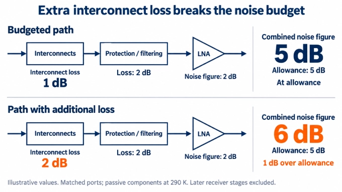
For this illustrative budget, assume matched ports at the operating frequency and passive input components at 290 K. The 5 dB noise-figure allowance covers the passive input network and LNA only; later receiver stages must be included separately in the cascade calculation.

Example input	Value
Noise-figure allowance for the passive input network plus LNA	5 dB
LNA noise figure	2 dB
Available loss allowance ahead of the LNA	3 dB
Illustrative allocation: protection/filtering	2 dB
Illustrative allocation: cables, connectors, and transitions	1 dB

If the installed interconnect loss increases from 1 dB to 2 dB, total passive loss ahead of the LNA rises from 3 dB to 4 dB. With the same 2 dB LNA noise figure, the combined noise figure becomes 6 dB, exceeding the 5 dB allowance.

Additional gain downstream cannot recover the lost signal-to-noise ratio. The engineer must reduce interconnect loss, reconsider LNA placement, or select lower-loss input components while preserving the required protection and interference rejection.

Usable Dynamic Range: Compression, Leakage, and Receiver Recovery

Usable dynamic range extends from the weakest input that meets detection requirements to the strongest signals the receiver can accommodate without unacceptable degradation. Both limits depend on the complete chain and the bandwidth under consideration.

Limitation	Consequence for the received signal
Gain compression	A strong input changes stage gain and distorts the response to weaker echoes.
Intermodulation	Strong signals generate unwanted products in nonlinear stages; some products can fall within the wanted band.
Excessive gain before a limited stage	A later amplifier, mixer, or ADC overloads even though earlier stages remain within their limits.
Transmitter leakage	Finite Tx/Rx isolation allows transmitted energy into the receiver, consuming headroom and potentially masking echoes.

Survival and usable reception are separate requirements. An input can remain below a damage limit while causing substantial compression or ADC clipping. Gain allocation must preserve headroom throughout the path while keeping downstream noise contributions acceptable.

In pulsed radar, the receiver must recover its specified gain, noise performance, and phase response before the earliest required echo arrives. Preventing damage alone does not guarantee sufficiently fast recovery.

CW and FMCW systems must accommodate leakage while receiving echoes. If leakage occupies the wanted receive band, an ordinary bandpass filter cannot selectively remove it. The required isolation therefore follows from actual transmit power, coupling paths, and receiver limits.

Phase Noise, Clock Jitter, and Waveform Fidelity

Spectral purity and waveform stability affect whether weak targets remain distinguishable near strong signals and whether the received waveform supports accurate measurements.

Phase noise: Noise skirts around strong returns or clutter can obscure weaker responses. LO phase noise can also mix with a strong blocker and raise noise within the wanted band, an effect called reciprocal mixing. Evaluate phase noise at relevant frequency offsets.
Sampling-clock jitter: Uncertainty in sampling instants introduces sample errors. Its effect becomes more severe as the ADC input frequency increases.
Waveform distortion: Amplitude variation and group-delay variation across the occupied band can distort compressed-pulse responses.

How Do Phased-Array and MIMO Radars Change RF Integration Requirements?

Phased-array and MIMO (Multiple Input, Multiple Output) radars require engineers to control relationships among channels as well as individual signal paths. In coherent arrays, relative amplitude, phase, and delay errors affect the combined result even when each channel meets its own specifications.

Approach	How signals are handled	Additional integration requirements
Analog or hybrid beamforming	Analog networks combine element signals. Hybrid systems also combine channels digitally, often across subarrays.	Control losses and relative gain and phase within the analog networks, then align the channels that remain separate.
Element-level digital beamforming	Each receiving element retains a separate digitized channel, and digital processing forms the beam.	Coordinate converters and sampling instants, characterize channel responses, and accommodate greater demands on connections, power, and cooling.
Co-located MIMO operation	Distinguishable transmitted signals allow echoes to be associated with transmit–receive pairs that form virtual channels.	Preserve the required timing, amplitude, and phase relationships, and maintain sufficient separation between transmitted signals and receive channels.

Phased-array beamforming and MIMO can coexist in one system. Multiple RF channels alone do not make a radar MIMO. For coherent operation, engineers allocate allowable differences in amplitude, phase, and delay according to their effect on beam direction, coherent gain, sidelobes, and angular estimates. Those limits must apply across the operating bandwidth and relevant array states, rather than only at one frequency or beam direction.

The LO and clock architecture must support coordinated operation across channels, including startup and mode changes. Calibration also needs physical access: reference inputs, sampling couplers, or observation paths must make channel responses accessible. Thermal gradients deserve particular attention because uneven heating can produce unequal gain and phase drift across the array, changing channel alignment during operation.

How Should Radar RF Interconnects Be Specified and Integrated?

In modular radar hardware, custom RF cable assemblies connect RF modules and antenna interfaces. Specify the loss, matching, delay, and power limits for the complete installed path, including mated connector pairs, PCB launches, and other transitions. In the earlier noise-budget example, the 1 dB interconnect allowance covers the combined loss of these connections ahead of the LNA.

Specification	What the requirement should establish
Frequency and interfaces	Define the operating band, impedance, and interfaces. Include the cable, connectors, and transitions in the assessment.
Insertion loss and return loss	Set maximum insertion loss and minimum return loss across the operating band for the assembled path.
Phase and delay	State allowable relative phase and group-delay errors, together with the frequency span and reference conditions.
Power handling	Specify peak and average power under the intended duty cycle, temperature, and load mismatch.
Shielding and grounding	Define shielding and interchannel coupling limits, including connector shells and ground continuity through transitions.
Mechanical installation	Set routing, bend-radius, strain-relief, and retention requirements, including repeatability after connector mating.

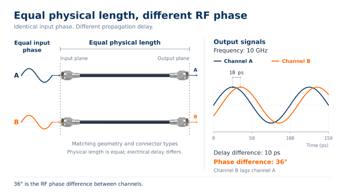
Phase matching and phase stability require separate limits. Matching describes agreement between assemblies under specified reference conditions. Stability describes how an assembly’s phase changes with temperature, bending, or movement. Equal physical lengths do not guarantee equal electrical lengths because dielectric properties, manufacturing variation, and connector terminations also affect propagation delay. Matching at one frequency also does not guarantee equal group delay across a wideband waveform.

Small delay differences can produce substantial phase errors. For a differential delay $\Delta\tau$ at frequency $f$ , the phase-error magnitude is:

|\Delta\phi| = 360^\circ f|\Delta\tau|

At 10 GHz, a 10 ps delay difference produces 36° of phase difference. The allowable delay difference must therefore follow the system’s phase budget.

Choose coaxial assemblies, PCB or board-to-board paths, or waveguide according to the operating band, power, loss, packaging, and service requirements.

How Are Radar RF Signal Paths Verified?

Verify RF performance at defined reference planes, with test cables and fixtures calibrated out or included deliberately. Use the specified operating band, waveform, signal levels, temperature, routing, and control states.

In the noise-budget example, check the input network’s insertion loss against the 3 dB allowance and the input-network-plus-LNA noise figure against the 5 dB allowance, under the stated reference conditions.

Requirement	Measurement	Relevant conditions
Gain, loss, matching, phase, and group delay	Use a suitable vector network analyzer (VNA) setup to characterize the RF response.	Cover the operating band, temperature range, and required control states.
Receiver sensitivity and strong-signal handling	Measure noise figure with a calibrated setup. Use signal generators to evaluate compression, intermodulation, and blocker response.	Apply specified wanted signals and interferers across relevant gain settings.
Transmit power and waveform quality	Use suitable RF power sensors and a signal analyzer to measure output power, waveform fidelity, harmonics, and spurious emissions.	Apply representative waveforms, duty cycles, loads, and temperatures.
Phase noise and timing	Measure phase-noise spectra and relevant clock jitter, skew, or synchronization timing.	Use actual carrier and clock frequencies, required offsets, and operating modes.
Tx/Rx isolation and recovery	Measure leakage and receiver response during and after representative transmit activity.	Reproduce pulse timing, power, coupling, and switching states.
Channel alignment and radiated performance	Compare channels using coherent stimuli, evaluate calibration residuals, and perform relevant over-the-air beam or target tests.	Cover representative beams, scan states, temperatures, and calibration states.

Frequency-converting or pulsed hardware may require synchronized sources and triggering. Component tests establish individual performance; assembled-path tests include installed connections and controls. System validation adds antenna behavior, calibration, and radiated responses. Record the configuration, conditions, uncertainty, and acceptance limits with the results.