Can One Assembly Be Replaced Without Rematching the Entire Set?

A replacement can be accepted using existing set data if those data still represent the retained assemblies. Verify the replacement against the applicable relationships, operating conditions, and acceptance rule. Changes to routing, connections, or correction settings may require additional checks. A matching part number alone does not establish interchangeability.

Do Phase and Delay Matching Also Guarantee Amplitude Matching?

No. Relative insertion loss requires its own limits across the applicable frequencies and operating conditions. Assemblies can satisfy phase and delay requirements while having different transmission magnitudes. If amplitude balance matters to the array budget, specify and verify it separately; phase and delay matching do not establish complete channel performance.

When Does Common Cable Delay Matter If Relative Delay Is Matched?

Delay shared by all channels leaves their relative timing unchanged. It still matters when the array must synchronize with another path, meet a latency requirement, or account for internal propagation delay in radar timing calibration. Specify absolute delay separately when those requirements apply; relative matching alone does not establish absolute timing.

Specifying Cable-Delay Matching Across a Phased Array’s Operating Band

Cable assemblies that agree in phase at one frequency can still introduce phase errors elsewhere in a phased array’s operating band. Equal physical lengths do not guarantee equal electrical delays, and a delay difference causes the relative phase to change with frequency.

A useful matching specification must therefore connect the array’s allowable channel error to limits on relative phase and, where needed, differential delay. Those limits need defined reference planes, operating conditions, and permitted corrections. This article develops that connection, then shows how to turn it into a cable requirement and verify the result.

Define What Must Be Matched, Where, and Over Which Band

A matched cable set must satisfy a defined relationship between electrical responses at specified reference planes. These planes mark the boundaries of the path being evaluated. Before assigning tolerances, establish what each response includes, which responses will be compared, and whether correction is permitted.

Measurement boundary: State whether the requirement covers complete connectorized assemblies or an installed RF path. Identify any adapters and fixtures included in that path.
Reference conditions: Identify the input and output connector interfaces that define the reference planes. State the reference impedance and transmission direction.
Frequency coverage: State the full operating range and the bandwidth used simultaneously under one correction state. Identify any subbands that use different correction settings.
Nominal relationship: State whether the paths should have equal phase and delay or specified intentional differences. Define those differences as functions of frequency where necessary.
Comparison basis: State whether limits apply between every pair of assemblies, between each assembly and a designated reference, or to deviations from nominal targets.
Permitted correction: State whether limits apply as delivered or after a fixed phase adjustment, a delay correction, or a frequency-dependent equalizer. Define each permitted correction explicitly.

The comparison basis changes what a tolerance guarantees. If each assembly can deviate by ±a from the same reference, two assemblies at opposite limits can differ by 2a. Set any reference-based tolerance so that it also satisfies the required pairwise limit.

For corrected performance, identify the correction the installed system can apply and how its settings are obtained. State whether one set of settings must cover the full band and operating conditions, or whether adjustment is allowed between subbands or after conditions change.

An assembly’s $S_{21}$ characterizes forward transmission under the declared S-parameter reference conditions. The installed channel response also depends on source and load mismatch and interactions with adjoining components. Assembly acceptance and installed-channel verification therefore need clearly defined boundaries.

Relate Phase Error to Differential Group Delay

Relative phase at one frequency establishes an offset between two paths. Differential RF group delay describes how that relative phase changes with frequency. These quantities describe different aspects of the same transmission response, so agreement in one does not establish agreement in the other.

Physical length measures geometry. Electrical phase length measures accumulated propagation phase: for an ideal matched transmission line of length $\ell$ , it is $\beta(f)\ell$ , where $\beta(f)$ is the phase constant. The transmission phase is the negative of that value. In a nondispersive line, phase changes linearly with frequency and group delay equals length divided by propagation velocity. In real assemblies, connector transitions and reflections at discontinuities also contribute to the measured phase response.

To compare assemblies, form the ratio $S_{21,i}(f)/S_{21,j}(f)$ at the defined reference planes and unwrap its phase continuously across frequency. Subtract the specified nominal phase difference to obtain the phase error, $e_{\phi,ij}(f)$ . The corresponding differential group-delay error is:

e_{\tau,ij}(f) = -\frac{1}{2\pi} \frac{d e_{\phi,ij}(f)}{df}

Use phase in radians, frequency in hertz, and delay in seconds. With this sign convention, a positive delay produces a negative phase slope. The delay error is positive when path i has more delay relative to path j than the nominal relationship specifies.

Integrating from a reference frequency gives:

e_{\phi,ij}(f) = e_{\phi,ij}(f_0) - 2\pi\int_{f_0}^{f}e_{\tau,ij}(\nu)\,d\nu

The phase error at any frequency therefore contains two contributions: the error at the reference frequency and the accumulated effect of differential delay between those frequencies.

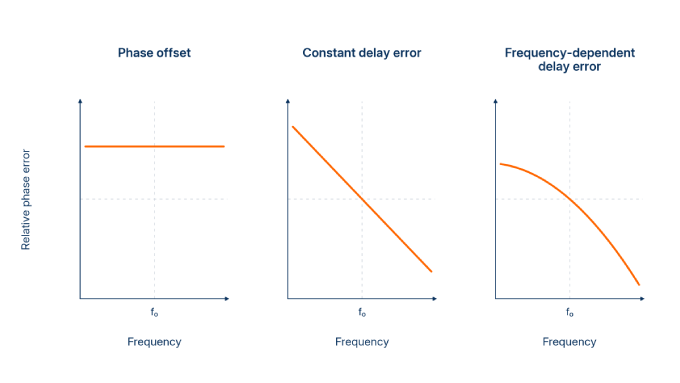
The term delay matching needs a more precise definition because it can refer to different metrics:

Local differential group delay: The difference between channel group delays at a particular frequency. Applied to phase error, the derivative above gives the corresponding delay error.
Fitted constant differential delay: The constant delay obtained from a linear fit to relative phase over a declared frequency interval, using a stated weighting.
Differential delay ripple: Variation in differential group delay relative to an explicitly defined baseline, such as a fitted constant delay.

When fitting the phase-error response, retain both the fitted delay error and its residual. Together, they describe the response before the fitted component was removed.

A single-frequency phase reading is ambiguous by whole multiples of $2\pi$ : matching readings can conceal different numbers of accumulated phase cycles. Matching group delay resolves a different issue, but still leaves a possible constant phase offset that requires a phase anchor.

The converse also matters. A phase-error curve can remain within a narrow envelope while varying rapidly with frequency. Its local slope—and therefore its differential group-delay error—can still be large. A phase envelope and a local delay limit consequently impose different constraints.

Allocate the Array Error Budget to the Cable Set

Allocate cable tolerances from the residual channel error the array can tolerate after intended steering and the permitted correction. First identify which spatial error patterns threaten the required performance. Then translate the cable share of that budget into phase and delay limits, accounting for the other channel components.

Connect Cable Error to the Required Array Performance

The spatial distribution of cable errors matters alongside their magnitude. A phase-only perturbation of the array factor shows where those errors enter:

AF(\hat{\mathbf u},f) = \sum_{n=1}^{N} a_n(f) \exp\left\{ j\left[ \frac{2\pi f}{c}\mathbf r_n\cdot\hat{\mathbf u} +\psi_n^{\mathrm{steer}}(f) +e_{\phi,n}(f) \right] \right\}

Here, $a_n$ is the amplitude weight, $\mathbf r_n$ is the element position, and $\hat{\mathbf u}$ is the observation direction. The intended excitation phase, $\psi_n^{\mathrm{steer}}$ , includes the steering law and nominal path compensation. The residual cable phase error, $e_{\phi,n}$ , is measured relative to a common reference.

Spatial error pattern	Principal consequence
The same phase error in every channel	Leaves relative alignment and array-factor magnitude unchanged at that frequency.
A linear phase gradient across the aperture	Shifts the beam; the shift depends on the phase gradient relative to the wavenumber.
Irregular channel errors	Alter coherent gain, sidelobes, and nulls according to their spatial structure.

Evaluate these effects over the required frequencies and scan states. Use bounded error patterns for a worst-case allocation, or declare the distributions and correlations used in a statistical allocation. An RMS phase value alone does not establish sidelobe performance. For wideband waveforms, also assess relative channel timing across the simultaneous bandwidth.

Keep cable errors separate from the steering architecture. Matched cables do not remove the beam squint associated with fixed-phase steering away from boresight. Re-tuning between operating frequencies differs from maintaining alignment across a simultaneous bandwidth under one steering state.

Convert the Phase Allocation Into a Usable Cable Requirement

Choose limits that match the system requirement and its available correction. A phase envelope directly constrains alignment at each frequency. A differential-delay limit can provide a conservative slope budget or impose an additional channel-timing requirement.

Consider a frequency-independent phase adjustment made at the center frequency and held fixed across the band. This adjustment removes a phase offset; it does not remove differential delay. Uncorrected paths do not receive that center-frequency subtraction, while paths with authorized delay correction must be assessed using their remaining delay error.

For constant differential delay and perfect center-frequency alignment, the largest phase-error magnitude occurs at the edges of a centered band:

|e_\phi|_{\max} = \pi B|\Delta\tau|

Here, $B$ is the full bandwidth. More generally, let $A$ bound the phase-error magnitude at the center frequency and let $D$ bound the magnitude of the total differential group-delay error throughout the band. The preceding integral relationship gives:

|e_\phi(f)| \le A + 2\pi D|f-f_0|

A sufficient condition for meeting a phase allowance $E_\phi$ across the centered band is therefore:

A + \pi B D \le E_\phi

This bound permits frequency-dependent delay. Because $D$ bounds the total delay error, its frequency variation is already included. If a limit instead applies only to a fitted constant delay, the remaining nonlinear phase needs a separate allowance.

Consider an illustrative 8–12 GHz requirement with phase alignment at 10 GHz and a 5° pairwise phase allowance. All values below are hypothetical, not iPrece performance guarantees.

After ideal center-frequency alignment, a constant 10 ps mismatch produces 7.2° of phase error at either band edge. It therefore exceeds the allowance. With zero center-frequency phase error, the largest permissible constant mismatch would be:

|\Delta\tau| \le \frac{5\pi/180}{\pi(4\times10^9)} \approx 6.94\ \mathrm{ps}

That ideal result leaves no allowance for imperfect phase alignment. Instead, allocate 1° to the residual center-frequency phase error and use 5 ps as the design bound on total differential group-delay error. The delay contribution is then at most 3.6°, giving a conservative phase bound of 4.6°.

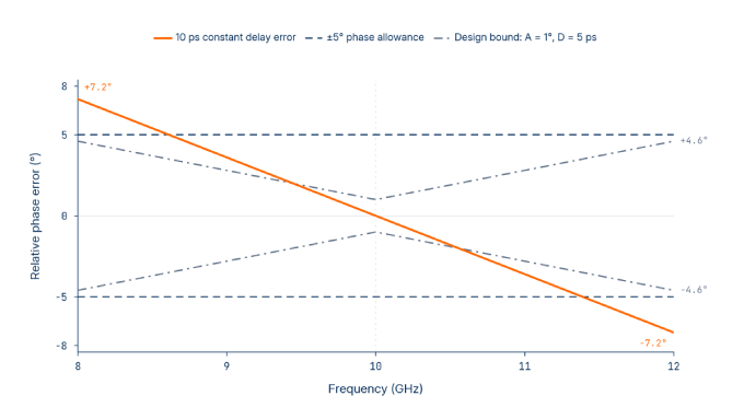
Calculated residual phase and conservative design bounds

Both allocations must apply to the corrected response being assessed. If the actual correction introduces additional frequency-dependent error, include that contribution before using the bound.

The following makes the phase envelope the controlling acceptance requirement. The 5 ps value remains a design allocation supporting the calculation.

Set and comparison basis: Apply the phase limits to every pair in an eight-assembly set. Identify each assembly by serial number.
Nominal relationship: The nominal targets are zero relative phase and zero differential delay after the permitted correction. Allow deviations within the stated acceptance limits.
Frequency range: Apply the requirement across 8–12 GHz under one correction state.
Phase acceptance limits: Require phase-error magnitude no greater than 5° across the band and 1° at 10 GHz after the specified correction.
Differential-delay design allocation: Use 5 ps as the pointwise bound on total differential group-delay error in the phase-budget calculation. This example does not impose it as a separate measured pass/fail limit.
Permitted correction: Allow one phase adjustment per channel, determined at 10 GHz and held fixed. For installed-performance acceptance, include the actual correction response and its residual errors. Do not remove individual assembly delays from the accepted response.
Cable measurement reference conditions: Measure each complete assembly between its two SMA mating planes, with a 50 Ω reference impedance, from end A to end B.
Acceptance condition: Stabilize the assemblies at 23 ± 1 °C in straight, supported, mechanically unstressed routes. Keep connections and routing unchanged after determining the phase adjustments.
Verification evidence: Supply calibrated complex cable transmission data, the correction values or characterized correction responses, and pairwise residual-phase results. Report delay estimates with their estimator and aperture. Record frequency spacing, temperature, routing, uncertainty, and acceptance disposition. Clearly distinguish calculated corrected responses from independently measured installed responses.

Verify the phase mask directly with adequate frequency resolution and the agreed uncertainty rule. Applying ideal phase rotations to cable data establishes the response under that mathematical correction model; installed-performance claims also require the actual correction response to be included.

If channel timing requires a separate delay acceptance limit, define the measured quantity, estimator, aperture, evaluation grid, and applicable conditions before testing. A finite-aperture result is an interval estimate of phase slope and does not automatically establish the pointwise derivative bound used in the calculation.

Require Matching to Hold Under Relevant Operating Conditions

Require evidence for conditions that occur in the application and can consume the allocated matching margin. The preceding example establishes initial matching under a controlled acceptance condition. It does not establish how the set will behave after installation or during temperature changes.

Distinguish three requirements. Initial matching establishes the relative responses in the reference condition. Environmental tracking describes how closely the assemblies change together as conditions vary. Return repeatability establishes whether their relative responses recover after an excursion.

Select the relevant assessments from the installation and service requirements:

Application condition	Reason for inclusion	Required test definition	Appropriate evidence stage
Reference condition	Establishes the baseline for the delivered set.	Define reference temperature, prior conditioning, routing, and the criterion for completing the soak.	Routine production acceptance.
Shared temperature changes	Establishes whether assemblies track when their temperatures change together.	Define temperature limits, ramps, dwell periods, and measurements at stabilized conditions.	Design or qualification characterization.
Unequal channel temperatures	Similar temperature responses can still produce unequal phase changes when assemblies experience different temperatures.	Reproduce relevant channel temperature differences and record individual assembly temperatures.	Qualification and installed-system verification.
Thermal excursion and return	Reveals hysteresis: the response at a given temperature can depend on thermal history.	Define excursion limits, sequence, cycle count, and measurements after returning to the reference condition.	Qualification characterization.
Installation and maintenance movement	Bends, restraints, and subsequent movement can change electrical response.	Define installed bend radii, support points, permitted movement, and the condition for the return measurement.	Qualification and installed-system verification.

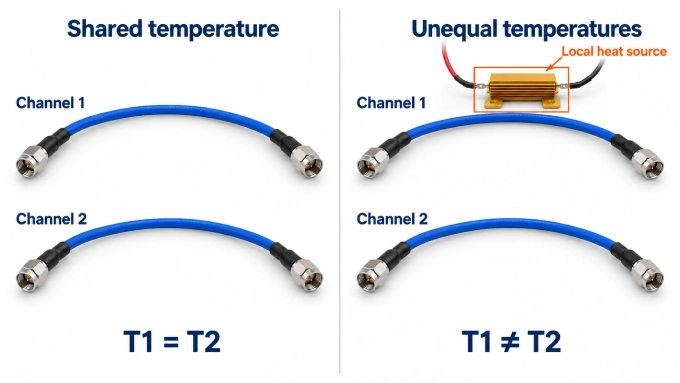
Thermal hysteresis and bend-induced phase changes make the assembly’s history and mechanical state relevant to phase stability. Apply the correction policy already specified: retain fixed settings throughout an excursion whenever the requirement prohibits recalibration. Define soak completion using assembly temperature stability, with response stability where needed, rather than chamber temperature alone.

Measure the specified relationships across the band. A phase-drift result at one frequency does not establish differential-delay tracking.

Qualification samples support production claims only through an explicit basis linking their construction and test results to controlled materials, manufacturing processes, and delivered-unit acceptance. Bulk-cable curves or another manufacturer’s normalized data cannot establish guarantees for the complete assemblies being supplied.

Consider iPrece ARX and Custom Assemblies for Your Cable Set

iPrece’s ARX phase-stable cables are a candidate when temperature changes or cable movement threaten channel alignment. Thermal and mechanical phase stability can help preserve an established match. Through iPrece’s custom RF cable assemblies, connector interfaces, cable construction, and lengths can be specified for the array’s layout.

Broadband matching must still be established for the finished connectorized assemblies. Support any matching claim with measured data from the actual set, demonstrating the required relative-phase and applicable delay performance across the operating band, at the declared reference planes and conditions.

Measure the Set and Make a Defensible Acceptance Decision

Demonstrating compliance requires comparable measurements at the declared reference planes, enough resolution to reveal relevant response features, and an agreed treatment of uncertainty. Apply the requirement already established, including its operating conditions and permitted correction, throughout measurement and acceptance.

Measure Complex Transmission Without Discarding the Specified Error

Preserve the assembly response at the declared reference planes and record every applied correction. Establish the measurement configuration before calibration, then confirm that the calibration remains applicable as the measurement is refined.

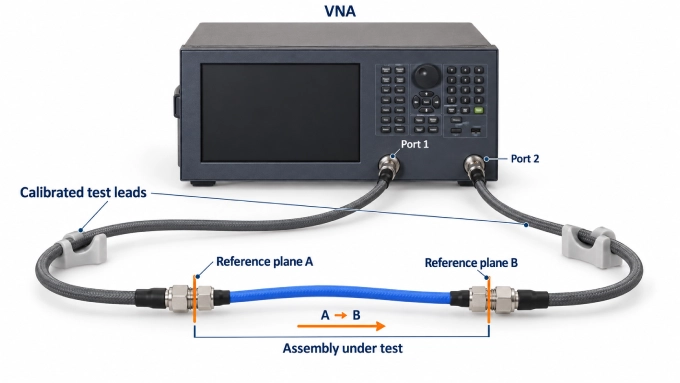
Confirm the configuration. Record assembly serial numbers, port orientation, routing, temperature, conditioning, and the permitted correction state.
Prepare and secure the setup. Inspect and clean mating interfaces, use the specified connector torque, and secure the test leads. Arrange connections so that changing assemblies causes as little movement of the calibrated leads as practicable.
Select the initial acquisition settings. Establish the sweep range, including any extension needed for delay estimates at the band edges. Choose an initial frequency grid, source power, IF bandwidth, and averaging. Use the longest expected electrical delay to select spacing that keeps the actual phase change between adjacent points below 180°, with margin.
Calibrate and verify. Perform an appropriate two-port calibration at the required planes. Where direct calibration is impractical, use a characterized fixture correction. Check the calibrated setup with an independent verification device before testing and repeat the check afterward to detect drift.
Acquire complex transmission. Measure calibrated $S_{21}$ for every assembly on a common frequency grid. Preserve the complex data before optional display processing.
Check frequency resolution. Repeat with finer spacing to confirm unwrapping and resolve relevant interior response features. When changing the sweep or stimulus settings, confirm that the calibration remains valid or recalibrate. Agreement at the band edges alone does not establish compliance between them.
Evaluate delay using the declared method. State the estimator, aperture in hertz, and any fitting or smoothing. Check whether narrower apertures reveal relevant features. At band edges, use a valid extended sweep or the explicitly specified alternative estimator; record any change in method.
Calculate the specified errors. Form the required relative responses, subtract the nominal relationship, and apply only the permitted correction. Repeat under the required operating conditions while retaining correction settings wherever specified.
Preserve the evidence. Save the calibrated data, serial-number mapping, settings, corrections, verification checks, and results. Retain full two-port data where installed-network analysis requires it.

A finite-aperture delay estimate represents phase slope over an interval. Increasing that interval reduces noise sensitivity while averaging response detail. Sampling and aperture checks must support the claimed resolution. Do not cover uncharacterized unresolved behavior with an arbitrary uncertainty allowance; characterize or bound it first. Quantified estimator and sampling effects can then be included in the uncertainty assessment.

Delay fitting is useful for diagnosis when the removed coefficients remain reported and assessed wherever required. Electrical-delay adjustment removes a linear phase term from a trace. Port extension moves the reference plane using a transmission-line model; fixture de-embedding uses a characterized network model. Delay-only port extension cannot remove arbitrary fixture mismatch.

Apply an Agreed Uncertainty and Acceptance Rule

A measured error inside tolerance is not automatically sufficient evidence of compliance. Its uncertainty may extend beyond the limit. Define the coverage interval and decision rule before testing, keeping measurement uncertainty separate from allowances for physical drift.

Build the uncertainty assessment for the relative quantity being accepted. Include:
Residual calibration errors and uncertainty in fixture corrections.
Reconnection, test-lead movement, reference stability, and drift.
Measurement noise and uncertainty associated with the defined phase or delay processing.

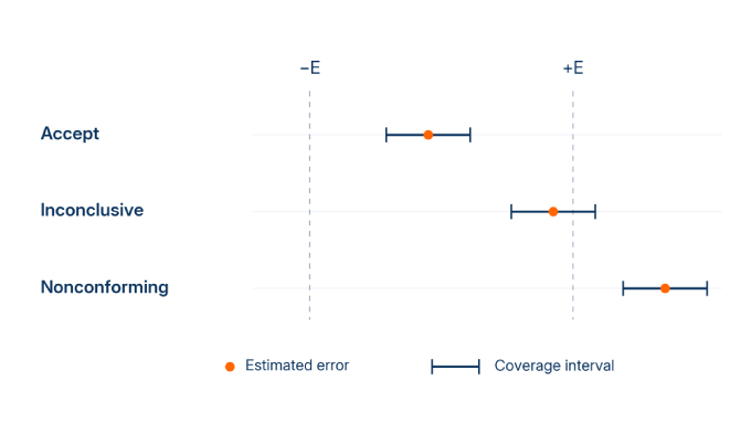
Coverage intervals inside, overlapping, or outside tolerance

Account for correlations between assembly measurements. Shared errors may cancel partly, while changes between measurements may remain. Assuming either complete cancellation or independence can misstate the uncertainty.

For an illustrative symmetric tolerance, let $\widehat e_q$ be the estimated error, $E_q$ the allowed magnitude, and $U_q$ the half-width of a symmetric coverage interval at a stated coverage probability. Here, $q$ denotes phase or a separately specified delay metric. One agreed rule is:

\text{Accept the result if}\quad |\widehat e_q| + U_q \le E_q

\text{Demonstrate nonconformity if}\quad |\widehat e_q| - U_q > E_q

These conditions place the coverage interval wholly inside or wholly outside tolerance, respectively. They illustrate guarded decisions consistent with conformity-assessment principles; they are not a universal cable standard.

Apply the rule to every required comparison, frequency, and condition:

Accept: All required results satisfy the acceptance condition.
Nonconforming: At least one result demonstrates nonconformity.
Inconclusive: Acceptance has not been demonstrated, but no result demonstrates nonconformity. Failure to satisfy the acceptance inequality alone belongs here.

Pointwise coverage does not automatically establish the same coverage probability for the complete frequency range and cable set. State the scope of the coverage claim explicitly.

Report the limits, worst results and their locations, uncertainty, tested conditions, applied corrections, exceptions, and final disposition. Identify both the measured errors and their margins after applying the decision rule.