What Is a Linear RF Amplifier? Linearity, Performance, & Applications Explained

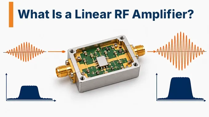
Linearity is a performance characteristic that can apply to many amplifier architectures. A Class A amplifier, Class AB amplifier, broadband gain block, low-noise amplifier, or power amplifier can be designed to satisfy particular linearity requirements.

Even architectures such as distributed RF amplifiers, which achieve broadband gain through multiple active devices connected along transmission lines, must be evaluated for compression, intermodulation, and other nonlinear behavior. Likewise, an amplifier's topology does not guarantee a specific level of linearity.

An amplifier with 30 dB gain is not necessarily more linear than one with 12 dB gain. Nor does a high saturated output-power rating guarantee low distortion at the intended operating point. The meaningful question is whether the amplifier meets the system's distortion limits at the required frequency, output power, bandwidth, and environmental conditions.

How Does a Linear RF Amplifier Work?

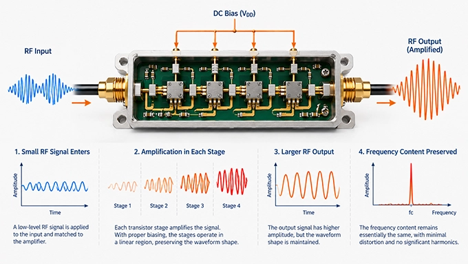
A linear RF amplifier operates within a region where its output signal remains approximately proportional to its input. Ideally, increasing the input amplitude by a given factor produces the same proportional increase at the output without introducing new frequency components.

For a simplified linear amplifier, the voltage relationship is:

Where:

• $Vout$ is the output voltage.

• $Vin$ is the input voltage.

• $Av$ is the voltage gain.

For example, an ideal amplifier with a voltage gain of 10 produces a 1 V output from a 100 mV input.

In a matched 50 Ω system, this corresponds to a power gain of 20 dB.

However, the relationship holds only within the amplifier's linear operating range. As the input signal increases, the transistor eventually approaches its voltage, current, or other device limitations. Gain becomes amplitude-dependent, and the output no longer follows the input proportionally.

What Happens When an RF Amplifier Becomes Nonlinear?

The output of a real amplifier can be approximated using a polynomial model:

Here, a₁ represents the linear response, while the higher-order terms describe nonlinear behavior.

The second-order term can generate second harmonics and second-order intermodulation products. The third-order term produces third harmonics and third-order intermodulation products.

This simplified model assumes a memoryless nonlinear system. Practical RF amplifiers can also exhibit memory effects caused by thermal behavior, bias networks, charge storage, and frequency-dependent impedances.

These effects make distortion dependent not only on instantaneous signal amplitude but also on the signal's recent history.

AM-AM and AM-PM Distortion

Two important manifestations of amplifier nonlinearity are AM-AM and AM-PM distortion.

• AM-AM distortion occurs when the amplifier's amplitude gain changes with input amplitude.

For example, a device may provide 15 dB gain at low input power but only 13 dB gain as it approaches compression.

• AM-PM distortion occurs when the amplifier's phase shift changes with input amplitude.

An input signal with a varying envelope can therefore experience different phase shifts at different instantaneous power levels.

Both effects are important in modern communication systems. AM-AM distortion changes the transmitted signal's amplitude relationships, while AM-PM distortion alters its phase relationships. Together, they can degrade modulation quality and create unwanted spectral components.

Why Is Linearity Important in RF Amplifiers?

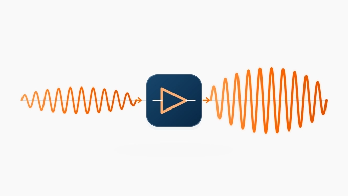
Linearity determines how accurately an amplifier preserves the information carried by an RF signal. A sufficiently linear amplifier increases signal power without introducing unacceptable amplitude distortion, phase distortion, or nonlinear mixing products. The consequences of poor linearity differ between transmitters and receivers.

Linearity in RF Transmitters

Modern transmitters frequently use modulation formats that carry information in both amplitude and phase. Examples include quadrature amplitude modulation (QAM) and orthogonal frequency-division multiplexing (OFDM).

These waveforms contain time-varying envelopes. When a power amplifier operates too close to compression, its nonlinear response changes the intended modulation.

The resulting impairments include:

• Constellation distortion and increased error vector magnitude

• Intermodulation products within and outside the occupied channel

• Spectral regrowth into adjacent frequency channels

• Increased adjacent-channel leakage

• Reduced modulation accuracy and potentially higher error rates

For example, a transmitter carrying a wideband OFDM signal may meet its average output-power requirement while failing its EVM or ACLR limits.

The problem is that average power alone does not describe how the amplifier handles instantaneous signal peaks.

Linearity in RF Receivers

Receiver linearity is particularly important when weak desired signals coexist with strong unwanted signals. Consider a receiver attempting to detect a weak signal at −90 dBm while two nearby interferers enter the receiver at considerably higher power levels. A nonlinear amplifier can mix these interferers and generate intermodulation products that fall inside the desired receive band. The resulting distortion may be difficult or impossible to remove with subsequent filtering because it occupies the same frequency range as the wanted signal. Strong blockers can also compress receiver gain, reducing the ability to detect weaker signals. This effect is commonly described as desensitization. For receiver design, low noise figure and high linearity must therefore be evaluated together. Noise figure determines how much the receiver degrades sensitivity at low signal levels, while compression and intermodulation performance constrain operation in the presence of strong signals.

Which Parameters Determine RF Amplifier Linearity?

RF amplifier linearity cannot be described adequately by a single specification. Different measurements reveal different nonlinear effects, and their importance depends on the signal waveform and operating conditions.

The following parameters are commonly used to evaluate RF amplifier distortion and linearity.

The critical distinction is that P1dB and IP3 characterize different aspects of nonlinear behavior, while EVM and ACLR evaluate the effects of distortion on actual modulated signals.

EVM: Measuring In-Band Signal Distortion

Error vector magnitude (EVM) measures the difference between the actual received or measured modulation symbols and their ideal reference positions in the complex I/Q plane.

EVM is commonly expressed as a percentage or in decibels.

A general RMS representation is:

The reference-power normalization depends on the applicable modulation standard or measurement definition.

For example, an RMS EVM of 4% indicates that the RMS error-vector magnitude is 4% of the specified reference amplitude.

A lower EVM generally indicates better modulation accuracy. However, EVM is not an exclusive measure of amplifier nonlinearity.

Noise, phase noise, IQ imbalance, frequency-response errors, and measurement-system impairments can also contribute to EVM. When evaluating an amplifier, engineers should characterize the input waveform and measurement setup so that the amplifier's contribution can be distinguished from other error sources.

ACLR: Measuring Adjacent-Channel Interference

Adjacent channel leakage ratio (ACLR) compares the integrated RF power in the intended transmission channel with the integrated power in a specified adjacent channel.

One common positive-ratio convention is:

For example, if the main-channel power is +23 dBm and the adjacent-channel power is −22 dBm:

The same result may be expressed as adjacent-channel power at −45 dBc relative to the main channel, depending on the reporting convention. An ACLR measurement must specify the channel bandwidths, adjacent-channel offsets, integration filters, and waveform conditions.

Unlike a two-tone IP3 measurement, ACLR directly evaluates the spectral behavior of a modulated signal. Poor RF amplifier linearity can increase spectral regrowth and degrade ACLR. However, phase noise and other transmitter impairments can also contribute to adjacent-channel leakage.

What Is the Difference Between P1dB, IP3, and Intermodulation Distortion?

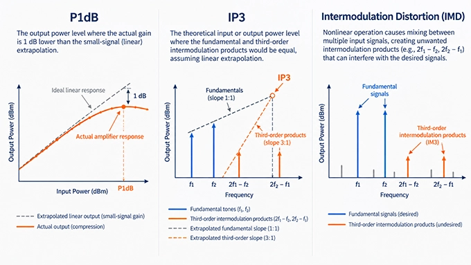
P1dB, IP3, and IMD are related to RF amplifier nonlinearity, but they describe different physical behaviors.

P1dB measures gain compression, IP3 characterizes the extrapolated relationship between fundamental signals and intermodulation products, and IMD measures distortion products under actual test conditions. Understanding the distinction is essential when comparing amplifier performance or calculating the linearity budget of an RF signal chain.

RF Amplifier P1dB: The 1 dB Compression Point

The 1 dB compression point is the input or output power level at which an amplifier's gain has fallen by 1 dB relative to its extrapolated small-signal gain.

It can be specified as:

• IP1dB: Input power at 1 dB compression

• OP1dB: Actual output power at 1 dB compression

Suppose an amplifier has a small-signal gain of 15 dB.

At an input power of −10 dBm, its expected linear output is:

As input power increases, the amplifier begins to compress.

Assume its input reaches +10 dBm, but the actual output is only +24 dBm instead of the +25 dBm predicted by constant 15 dB gain.

The amplifier is now at its 1 dB compression point.

Therefore:

P1dB provides a useful indication of large-signal capability. However, operation below P1dB does not guarantee acceptable EVM, ACLR, or intermodulation performance.

A demanding modulation format may require substantially more output-power back-off.

RF Amplifier IP3: The Third-Order Intercept Point

IP3 characterizes the third-order nonlinear response of an amplifier, generally using a two-tone test.

Two closely spaced sinusoidal signals are applied to the input:

A nonlinear amplifier generates intermodulation products at frequencies including:

These third-order products are particularly important because they appear close to the original tones and can fall within the operating band.

In the small-signal cubic approximation, fundamental output power increases by approximately 1 dB for every 1 dB increase in input power.

Third-order intermodulation products increase by approximately 3 dB for the same input-power increase.

If both responses are extrapolated, their theoretical intersection defines IP3.

Two reference points are used:

1. IIP3 (Input IP3): The hypothetical intercept referred to the amplifier input.

2. OIP3 (Output IP3): The hypothetical intercept referred to the amplifier output.

For an amplifier with small-signal gain G in dB:

IP3 is not an actual operating power limit.

The mathematical intersection normally lies outside the region where the low-level cubic approximation remains valid. The amplifier may already be heavily compressed before reaching that extrapolated power.

Intermodulation Distortion (IMD)

Intermodulation distortion refers to unwanted frequency components generated when two or more signals interact through a nonlinear system.

For two equal-amplitude input tones, the third-order intermodulation level can be related to OIP3.

Under the conventional weakly nonlinear approximation:

Here, Pout, tone is the output power of either fundamental tone in dBm.

The result is the power of an individual third-order intermodulation product relative to its corresponding fundamental tone.

The approximation assumes equal-amplitude input tones, approximately cubic nonlinear behavior, and operation sufficiently below compression.

Worked Example: Calculating OIP3 and IMD3

Consider a 2.4 GHz RF amplifier with the following assumed characteristics:

Step 1: Calculate the third-order frequencies.

The lower third-order product appears at:

The upper third-order product appears at:

Step 2: Calculate the relative IMD3 level.

Each fundamental tone has an output power of +10 dBm, while each third-order product is measured at −40 dBm.

Each intermodulation product is therefore 50 dB below its corresponding fundamental.

Step 3: Calculate OIP3.

For the conventional equal-tone extrapolation:

Step 4: Calculate IIP3.

The resulting intercept specifications are:

• $\mathrm{OIP3} = +35\,\mathrm{dBm}$

• $\mathrm{IIP3} = +20\,\mathrm{dBm}$

• $\mathrm{IMD3} = -50\,\mathrm{dBc}\ \text{at}\ +10\,\mathrm{dBm}\ \text{output per tone}$

These values are internally consistent under the assumed weakly nonlinear conditions.

They do not establish the amplifier's P1dB, maximum safe input power, or modulated-signal ACLR.

Can P1dB and IP3 Be Used Interchangeably?

No. Although P1dB and IP3 may correlate for some amplifier designs, no universal conversion accurately relates them across all devices.

P1dB is determined from gain compression, usually with a single-tone input.

IP3 is extrapolated from intermodulation measurements, usually using two tones.

Two amplifiers with similar P1dB ratings may have different IP3 values, especially if they use different transistor technologies, feedback networks, bias conditions, or linearization techniques.

Engineers should use the specification that corresponds to the distortion mechanism relevant to the application.

How Do RF Amplifier Linearity and Efficiency Trade Off?

An RF amplifier generally becomes less linear as it approaches its maximum available output power.

Operating farther from compression improves signal fidelity, but it often reduces power efficiency.

This creates one of the central trade-offs in RF power amplifier design.

How Amplifier Bias Class Affects Linearity

Amplifier operating classes describe how the active device conducts current during an RF cycle.

Class A operation keeps the active device conducting throughout the RF cycle.

This typically provides favorable intrinsic linearity, but substantial DC power is consumed even when the RF output is small.

Class AB reduces the conduction angle and quiescent current, improving efficiency while introducing greater nonlinear behavior.

Class B and C operation can further reduce conduction time, but their current waveforms contain stronger nonlinear components.

These are general tendencies, not absolute performance rankings.

For example, a carefully designed Class AB power amplifier with linearization may meet stringent modulation requirements while achieving higher efficiency than a Class A implementation.

Similarly, a Class A amplifier is not perfectly linear at every input power or frequency.

Output Back-Off and Modulated Signal Peaks

A common way to improve linearity is to reduce the average RF output power relative to the amplifier's compression or saturation level.

This is known as output power back-off.

For example, suppose an amplifier has:

• $\mathrm{OP_{1dB}} = +30\,\mathrm{dBm}$

• $\text{Average RF output power} = +18\,\mathrm{dBm}$

The average output-power back-off relative to OP1dB is:

The amplifier operates well below its single-tone compression point on an average-power basis.

However, a modulated waveform can contain substantial instantaneous peaks.

If the waveform has an observed peak-to-average power ratio (PAPR) of 8 dB, its corresponding peak output power is approximately:

The peaks are only 4 dB below the amplifier's OP1dB.

Whether this margin is sufficient depends on the actual AM-AM and AM-PM response, waveform statistics, and required EVM and ACLR.

A single-tone compression point cannot, by itself, establish acceptable performance with a modulated waveform.

How Digital Predistortion Improves Linearity

Digital predistortion (DPD) is a technique used to compensate for predictable nonlinear behavior.

Instead of requiring the amplifier itself to be highly linear at every operating point, the input waveform is deliberately modified before amplification.

For example, if the amplifier compresses large signal amplitudes, the predistortion system can apply an opposing amplitude characteristic.

Similarly, predistortion can compensate for amplitude-dependent phase shifts.

The objective is for the combination of predistorter and amplifier to produce an approximately linear overall response.

Modern DPD implementations may use memory polynomial or related nonlinear models to compensate for both instantaneous distortion and memory effects.

DPD can improve EVM and ACLR and may allow an amplifier to operate more efficiently at higher average power.

However, predistortion has limitations.

It requires sufficient signal-generation bandwidth, measurement feedback or model accuracy, and usable amplifier headroom. It cannot perfectly recover information that has been irreversibly clipped by severe saturation.

Other Techniques for Improving Linear Efficiency

Several amplifier architectures and control techniques attempt to improve efficiency without sacrificing required modulation performance.

• Doherty amplification: Uses load modulation to improve efficiency over a range of output power levels, particularly under backed-off operation.

• Envelope tracking: Adjusts the amplifier supply voltage in response to the signal envelope to reduce unnecessary power dissipation.

• Feedback and feedforward linearization: Use correction signals or feedback mechanisms to reduce nonlinear distortion.

• Bias optimization: Adjusts transistor operating conditions to balance efficiency, gain, and distortion.

Each technique introduces its own limitations involving bandwidth, complexity, stability, control accuracy, or implementation cost.

The appropriate method depends on the waveform and system-level linearity requirements.

What Is the Difference Between Linear and Nonlinear RF Amplifiers?

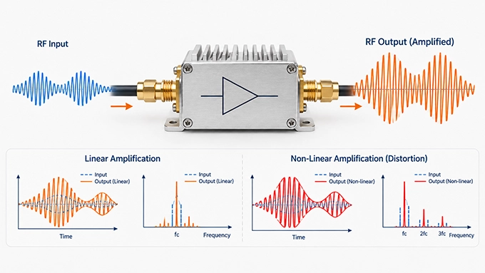
The terms linear and nonlinear describe an amplifier's operating behavior, not necessarily two completely separate circuit architectures.

Every practical RF amplifier exhibits some nonlinearity.

An amplifier is considered sufficiently linear when its gain and phase response preserve the intended signal within the application's specified distortion limits.

A nonlinear amplifier, or an amplifier operating in a strongly nonlinear region, no longer maintains this proportional relationship.

Is a Linear RF Amplifier a Separate Circuit Topology?

Not necessarily.

Linearity is a performance characteristic that can apply to many amplifier architectures.

A Class A amplifier, Class AB amplifier, broadband gain block, low-noise amplifier, or power amplifier can be designed to satisfy particular linearity requirements.

Even architectures such as Distributed RF Amplifiers, which achieve broadband gain through multiple active devices connected along transmission lines, must be evaluated for compression, intermodulation, and other nonlinear behavior.

Likewise, an amplifier's topology does not guarantee a specific level of linearity.

An amplifier with 30 dB gain is not necessarily more linear than one with 12 dB gain. Nor does a high saturated output-power rating guarantee low distortion at the intended operating point.

The meaningful question is whether the amplifier meets the system's distortion limits at the required frequency, output power, bandwidth, and environmental conditions.

Where Are Linear RF Amplifiers Used?

Linear amplification is important in RF systems where distortion can affect information accuracy, receiver sensitivity, adjacent-channel interference, or measurement integrity.

Wireless Communication Transmitters

Cellular base stations and broadband wireless transmitters use linear amplification to preserve complex modulation formats such as QAM and OFDM. EVM, ACLR, output power, and efficiency are central performance requirements in these applications.

Satellite Communication Systems

Satellite communication transmitters and ground terminals use amplifiers that must control nonlinear distortion when carrying amplitude- and phase-modulated signals. Output back-off and linearization are especially relevant when high-power amplification is required.

RF Receiver Front Ends

Low-noise amplifiers and intermediate gain stages require adequate linearity to handle strong blockers without excessive intermodulation or gain compression. Receiver design must balance noise figure, gain, IP3, and compression performance.

Radar and Wideband Signal Processing

Radar systems can require controlled amplitude and phase behavior for wideband waveforms, pulse compression, and coherent processing. The necessary linearity depends on the waveform, modulation, dynamic range, and signal-chain architecture.

RF Test and Measurement Equipment

Signal generators, measurement receivers, and broadband test systems rely on linear gain stages to avoid adding distortion that could be mistaken for device-under-test behavior. High linearity supports accurate characterization of signals and components.

How Should RF Engineers Select a Linear Amplifier?

Selecting a linear amplifier requires more than comparing gain and maximum output-power ratings.

The amplifier must satisfy the system's distortion limits under the intended operating conditions, including frequency, waveform, temperature, impedance matching, and power level.

1. Define the Signal and Operating Frequency Range

Begin with the required frequency band, modulation format, instantaneous bandwidth, and signal levels.

For example, a transmitter operating from 2.40 to 2.50 GHz with a 20 MHz modulated waveform may have different linearity requirements from a continuous-wave transmitter using the same frequency range.

Specify the characteristic impedance and expected source and load conditions.

2. Establish Gain and Output-Power Requirements

Determine the available RF input power and the required output power.

For a matched system, the basic gain relationship is:

For example, increasing an input signal from −5 dBm to +15 dBm requires 20 dB gain.

However, this calculation determines only the nominal gain requirement.

It does not show whether the amplifier can deliver +15 dBm without unacceptable distortion.

3. Calculate the Required Linearity Margin

Establish the acceptable compression and intermodulation limits at the intended operating point.

For a modulated waveform, consider both average output power and peak-to-average power ratio.

As an illustrative case, assume:

The candidate provides only 1 dB of separation between the observed peak power and its single-tone OP1dB.

That is not sufficient evidence that the amplifier will meet strict EVM or ACLR requirements.

A device with a higher compression point may provide more headroom, but final acceptance still depends on modulated-signal measurements.

4. Evaluate IP3 and Intermodulation Performance

For receiver applications, assess IIP3 relative to expected blocker power levels.

For transmitters and driver stages, OIP3 can help estimate low-level intermodulation performance.

When comparing specifications, verify whether the intercept point is input- or output-referred.

Also check the test frequency, tone spacing, output power, bias, and temperature.

An IP3 value obtained at one test condition should not automatically be treated as valid over a different operating band or power range.

5. Verify EVM and ACLR With the Intended Waveform

For digitally modulated signals, evaluate the amplifier using representative modulation and bandwidth conditions.

Specify the required EVM and ACLR limits and measure performance at the intended average output power.

For example, a particular system design might require:

These are illustrative engineering targets, not universal standards applicable to all RF systems.

The actual acceptance criteria must follow the communication standard or system specification.

Measurements should also distinguish amplifier-generated distortion from impairments already present in the test signal.

6. Evaluate Efficiency, Bias, and Thermal Conditions

A highly linear amplifier may still be unsuitable if its power consumption or thermal dissipation exceeds system limits.

Power-added efficiency is commonly expressed as:

All powers in this expression must be in watts.

Evaluate efficiency at the required average output power—not only at the amplifier's maximum-power operating point.

Bias current, supply voltage, device temperature, and thermal impedance should be included in the assessment.

For high-power systems, determine whether output back-off, digital predistortion, or a more efficient amplifier architecture is required.

7. Verify Performance in the Complete RF Signal Chain

The final evaluation should include the amplifier's installed RF environment.

Connectors, PCB transmission lines, matching networks, and custom rf cable assemblies can introduce loss, mismatch, and frequency-dependent phase variation.

Although passive interconnects are generally linear under normal conditions, their losses and mismatches can alter the power delivered to the amplifier or the load.

A vector network analyzer can characterize small-signal gain and port matching. A signal generator, spectrum analyzer or vector signal analyzer, and appropriate RF power measurements are needed to evaluate compression, intermodulation, EVM, and ACLR.

Test-fixture effects should be calibrated or de-embedded as appropriate.

When evaluating output matching, distinguish small-signal RF amplifier output impedance from the optimum load impedance required for high-power operation.

The final acceptance test should reproduce the actual frequency, waveform, bias, temperature, and load conditions as closely as practical.

Practical Measurement Checklist

Before accepting an amplifier's linearity measurements, verify that:

• The signal generator's own distortion is sufficiently below the required measurement level.

• Two-tone sources are adequately isolated to prevent source-generated intermodulation.

• The analyzer input is protected from excessive RF power and is not generating significant distortion of its own.

• Cable, attenuator, and fixture losses are included in the measurement reference planes.

• EVM and ACLR measurement bandwidths and settings match the intended signal standard.

• Bias voltage, quiescent current, and operating temperature are recorded.

• Linearity is checked at the required power level rather than inferred only from datasheet maxima.

The objective is to measure the amplifier's actual nonlinear behavior, rather than distortion originating in the test setup.