Distributed Power RF Amplifiers for RF And Microwave Commiunications

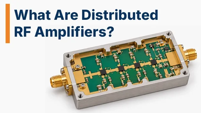
Distributed RF amplifiers achieve broadband gain by connecting multiple active devices along two transmission lines rather than cascading them through conventional interstage matching networks. This architecture allows the transistors' parasitic capacitances to become part of the transmission-line structure, reducing their usual bandwidth-limiting effect.

However, wide bandwidth introduces trade-offs involving gain, noise figure, power efficiency, and phase matching. Understanding how signals propagate through the gate and drain lines (and how their contributions combine at the output) is essential for evaluating distributed amplifier performance.

Understanding Distributed RF Amplifiers

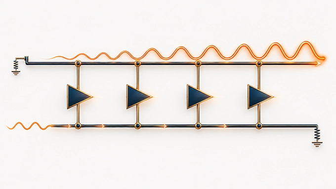
A distributed RF amplifier is a broadband amplifier topology that combines the output contributions of multiple active devices through phase-matched transmission lines. Also called a distributed amplifier (DA) or traveling-wave amplifier, it uses separate input and output transmission lines to distribute the RF signal and collect amplified contributions.

In a conventional multistage amplifier, the output of one gain stage drives the input of the next. In a distributed amplifier, several transistors are connected along common transmission-line structures.

For a typical field-effect transistor (FET) implementation:

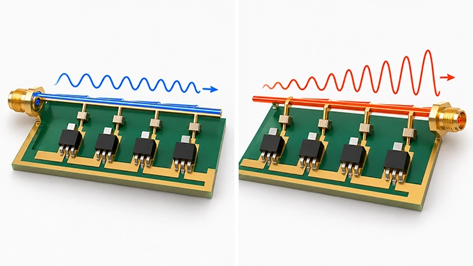
• The gate transmission line distributes the input RF signal to successive transistor gates.

• The drain transmission line collects the amplified current contributions from the transistor drains.

• The active devices convert local RF gate-voltage variations into drain-current variations.

• The termination networks absorb unwanted traveling waves and reduce reflections.

The transmission lines are designed so that the amplified signals from successive transistors arrive at the output with approximately the same phase.

This constructive signal combination provides gain across a wider frequency range than would generally be practical with an equivalent arrangement relying on conventional narrowband matching networks.

The distributed principle is not limited to FETs. Bipolar transistor implementations use corresponding input and output electrodes, such as base and collector nodes.

Is a Distributed Amplifier the Same as a Traveling-Wave Amplifier?

The terms are often used interchangeably in solid-state microwave amplifier design.

Both describe architectures in which an RF signal propagates along a structure and interacts with multiple active gain elements.

However, a solid-state distributed amplifier should not be confused with a traveling-wave tube amplifier (TWTA).

A TWTA is a vacuum-electronic device that amplifies RF signals through interaction between an electron beam and an electromagnetic wave propagating along a slow-wave structure.

Although both technologies exploit wave propagation, their physical operating mechanisms are fundamentally different.

How Does a Distributed RF Amplifier Work?

The distributed amplifier working principle relies on propagating the input signal through successive gain cells while combining their amplified outputs coherently along a second transmission line.

Consider a conventional distributed FET amplifier containing four identical transistor stages.

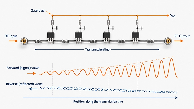
The signal enters the gate line and travels toward its termination. As the traveling wave reaches each transistor, the local gate voltage produces an RF drain current.

For a simplified small-signal transistor model:

Where:

• $i_d,k$ is the RF drain-current contribution of stage k.

• $g_m,k$ is its small-signal transconductance.

• $v_gs,k$ is the RF gate-to-source voltage at that stage.

Each transistor injects a current wave into the drain transmission line.

That excitation launches waves traveling in both directions along the drain line. The forward-traveling contributions propagate toward the output, while the backward-traveling components propagate toward the drain termination.

The drain and gate transmission lines are designed to maintain the correct timing relationship between these contributions.

How Do Signals Combine Constructively?

Suppose the RF signal reaches transistor 1 first, causing it to inject an amplified current into the drain line.

The output contribution from transistor 1 then travels toward transistor 2.

If the propagation delay between the first and second gate connections matches the corresponding drain-line delay, the contribution from transistor 1 arrives at the second drain connection as transistor 2 generates its own amplified current.

The two contributions add constructively and The process repeats through the remaining stages.

Ideally, the total forward-traveling output wave is the coherent sum of the contributions from all transistors.

For identical gain cells, matched transmission lines, and negligible losses, the approximate voltage gain is:

Where:

• $N$ = number of active gain cells

• $g_m$ = transconductance of each transistor, in siemens

• $Z_d$ = characteristic impedance of the drain transmission line

The factor of 1/2 appears because a current injected into an ideal, matched drain line initially divides between the forward and backward propagation directions.

This is a simplified low-frequency, small-signal approximation. It assumes phase-matched propagation, identical devices, negligible transmission-line attenuation, and suitable input and output matching.

Under these assumptions, voltage gain scales approximately with the number of stages, while power gain scales approximately with N².

Real distributed amplifiers do not continue gaining indefinitely as stages are added. Transmission-line attenuation, phase errors, loading and device limitations eventually reduce the benefit of additional gain cells.

Why Are Termination Resistors Necessary?

A conventional distributed amplifier generally has two important terminations.

1. Gate-line termination: Located beyond the final input-stage connection, this termination absorbs the remaining forward-traveling input wave and reduces reflections back toward the source.

2. Drain-line termination: Located at the end opposite the RF output, this termination absorbs backward-traveling drain-line waves.

These terminations support broadband matching and suppress reflections that could disturb the intended signal combination.

They also introduce trade-offs.

The drain termination dissipates RF power, reducing efficiency. The gate termination introduces thermal noise that contributes to the amplifier's overall noise figure.

An important distinction is that backward-traveling drain waves are not necessarily eliminated through perfect cancellation. The termination provides a matched path for absorbing them.

What Are Gate and Drain Transmission Lines in a Distributed Amplifier?

The gate and drain transmission lines are the defining components of a distributed amplifier architecture.

They are not simply interconnects between transistors. Their impedance, propagation delay, attenuation, and parasitic loading determine how effectively the amplifier combines gain over frequency.

Gate Transmission Line: Distributing the Input Signal

The gate transmission line carries the incoming RF signal past the inputs of successive gain cells.

In a FET implementation, each gate presents capacitance to the line, primarily associated with the gate-source capacitance, Cgs.

Additional parasitic capacitances, including gate-drain capacitance, can also affect the effective input loading.

In a conventional amplifier, transistor input capacitance combines with the surrounding impedance to create frequency-dependent attenuation and phase shift.

A distributed amplifier instead incorporates this capacitance into a transmission-line structure.

A simplified artificial gate line consists of:

• Series inductance between adjacent gain cells

• Shunt capacitance associated with the transistor inputs

• Additional parasitic capacitances and resistive losses

• A termination matched to the line's effective characteristic impedance

The series inductances may be implemented using lumped inductors or suitable high-impedance transmission-line sections.

Together with the device capacitances, these elements approximate a periodically loaded transmission line.

Drain Transmission Line: Combining the Amplified Signals

The drain transmission line performs a different function.

Rather than distributing an external signal to the transistors, it collects the RF current generated by their drain terminals.

Each transistor contributes a controlled current source to the drain line.

The drain-line network incorporates:

• Series inductance between gain cells

• Transistor drain capacitance and additional output loading

• Drain conductance and associated losses

• RF output and reverse-wave termination networks

The effective drain-line impedance influences the voltage developed by the injected current.

However, increasing drain-line impedance is not an unrestricted way to increase gain. It also affects matching, voltage swing, power handling and the phase relationship with the gate line.

What Are Artificial Transmission Lines?

An artificial transmission line is a network of periodically repeated inductive and capacitive elements that approximates a continuous transmission line over a limited frequency range.

For an ideal lossless LC ladder, with series inductance L and shunt capacitance C per repeated section, the approximate low-frequency characteristic impedance is:

The propagation delay per section is approximately:

For a conventional symmetric periodic LC ladder, the theoretical upper passband edge is:

These relationships are useful for preliminary design, but they do not fully describe a practical distributed amplifier.

Real transistor capacitances are frequency- and bias-dependent, transmission-line elements have losses, and periodic structures exhibit dispersion as frequency approaches cutoff.

The practical amplifier bandwidth can therefore be significantly lower than the calculated ideal LC cutoff.

Why Must Gate and Drain Propagation Delays Match?

Constructive amplification requires the RF contributions from different stages to reach the output with the intended phase relationship.

For a periodic distributed amplifier, the phase shift per corresponding gate and drain section should approximately satisfy:

Where:

• $β_g$ and $β_d$ are the phase constants of the gate and drain lines.

• $l_g$ and $l_d$ are the lengths of their corresponding sections.

In an ideal low-loss artificial-line model, this is related to matching the per-section propagation delays:

The effective gate and drain capacitances are rarely identical.

Consequently, designers may adjust the line inductances, introduce additional capacitance, or modify the gain-cell structure to obtain suitable phase matching.

The objective is not simply to make the two transmission lines physically equal in length. Their electrical phase shifts must be coordinated across the intended operating band.

Why Do Distributed RF Amplifiers Provide Wide Bandwidth?

The main reason distributed RF amplifiers provide wide bandwidth is that transistor parasitic capacitances are incorporated into transmission-line structures instead of being treated only as localized capacitive loads.

How Parasitic Capacitance Limits Conventional Amplifiers

In a simplified conventional amplifier, a transistor capacitance interacting with a resistance introduces a frequency-dependent pole.

For an elementary RC network:

Increasing capacitance or resistance lowers the corresponding cutoff frequency.

Practical transistor amplifiers are more complicated because they include feedback capacitances, matching networks, multiple poles, and frequency-dependent device characteristics.

Nevertheless, the underlying problem remains: parasitic capacitances increasingly affect gain and phase at high frequencies.

How Distributed Amplification Changes the Limitation

In a distributed architecture, the transistor capacitances become part of periodically loaded gate and drain lines.

Instead of driving a single concentrated capacitive load, the input wave propagates through a network whose inductive and capacitive elements are distributed among successive gain cells.

This changes how the capacitances affect the frequency response.

Properly designed lines can transmit the RF excitation across a broad passband while maintaining the phase relationship required for constructive output combining.

The approach can support broadband gain across multiple octaves and in suitable implementations, frequency ranges spanning more than one decade.

However, distributed amplification does not eliminate transistor parasitics or create unlimited bandwidth. It incorporates some of their effects into a more favorable circuit structure.

What Actually Limits Distributed Amplifier Bandwidth?

Several mechanisms ultimately restrict the usable bandwidth.

1. Artificial transmission-line cutoff

The gate and drain networks have finite passbands. Their propagation and impedance characteristics become increasingly dispersive near their cutoff frequencies.

2. Transistor high-frequency performance

Device transconductance, intrinsic capacitances, transit-time effects, and transistor frequency limits constrain the gain available at high frequencies.

The transistor transition frequency, fT, and maximum oscillation frequency, fmax, are useful technology indicators, but neither directly equals the amplifier's operating bandwidth.

3. Transmission-line attenuation

Metal resistance, skin effect, dielectric loss, and substrate effects increase attenuation along the gate and drain lines.

These losses reduce the excitation reaching later stages and the amplified contributions reaching the output.

4. Phase mismatch

Differences between gate-line and drain-line propagation introduce phase errors that prevent ideal coherent combining.

5. Input and output matching

The effective impedance of the loaded lines changes with frequency. Mismatch and reflections can introduce gain ripple and reduce the usable operating range.

6. Packaging and bias networks

RF launches, bond wires, interconnects, DC-blocking capacitors, and bias structures can introduce additional poles, resonances, and low-frequency restrictions.

The practical bandwidth is therefore determined by the complete active and passive network rather than any single cutoff parameter.

Worked Example: Estimating Gain and Artificial-Line Bandwidth

Consider a simplified four-stage distributed FET amplifier.

Assume the following idealized small-signal parameters:

Step 1: Calculate the characteristic impedance

Using the ideal LC approximation:

Both artificial lines therefore have an approximate low-frequency characteristic impedance of 50 Ω.

Step 2: Estimate the propagation delay

Because the assumed effective L and C values are equal for the gate and drain lines, their ideal section delays are matched.

Step 3: Estimate the ideal LC cutoff

This is the theoretical cutoff of the simplified LC ladder, not the guaranteed operating bandwidth of the amplifier.

Step 4: Estimate ideal small-signal voltage gain

Using the lossless distributed gain approximation:

With equal 50 Ω input and output reference impedances and ideal matching:

The approximate result is therefore 12 dB of small-signal gain under the stated ideal conditions.

In a practical design, finite transistor bandwidth, transmission-line attenuation, phase mismatch, and parasitic loading reduce or reshape the gain response.

A nonlinear transistor model and electromagnetic simulation of the passive structures would be required before claiming a realizable 12 dB gain or a specific operating frequency range.

Which Parameters Determine Distributed Amplifier Performance?

A distributed amplifier should be evaluated as a broadband active two-port network.

The most important parameters describe its gain, frequency response, noise contribution, linearity, power capability, impedance matching, stability, and DC power requirements.

Small-Signal Gain and Gain Flatness

Small-signal gain describes how much the amplifier increases signal power while operating within its linear region.

For a matched two-port measurement:

The gain is frequency-dependent because transistor transconductance, line attenuation, phase matching, and impedance matching vary over the passband.

Gain flatness describes the variation in gain across the required operating range.

For example, an amplifier with gain ranging from 10 dB to 12 dB over its specified band has 2 dB peak-to-peak gain variation.

Gain flatness is particularly important when the amplifier must support wideband signals without introducing substantial frequency-dependent amplitude distortion.

Distributed designs may exhibit negative gain slope at high frequencies due to increasing line losses. Gain-cell sizing, line tapering, and other circuit-level techniques can be used to reshape this response.

Distributed Amplifier Bandwidth

Bandwidth defines the frequency range over which the amplifier satisfies its specified performance requirements.

The usable bandwidth may be limited by:

• Minimum acceptable small-signal gain

• Maximum permitted gain ripple

• Input and output matching

• Noise-figure requirements

• Output power or linearity

• Stability constraints

The 3 dB gain bandwidth is a common characterization, but it is not necessarily the system's usable bandwidth.

For example, a circuit may maintain gain within 3 dB over a wide frequency range while failing a stricter ±1 dB flatness requirement.

Therefore, distributed amplifier bandwidth should always be associated with a clearly defined acceptance criterion.

Noise Figure

Noise figure quantifies the degradation in signal-to-noise ratio introduced by an amplifier.

It is related to the linear noise factor F by:

Distributed amplifiers have multiple noise contributors, including the transistor channels, gate and drain structures, resistive losses, and termination networks.

The gate-line termination is particularly important because its thermal noise can couple through the distributed gain cells and reach the output.

In conventional distributed architectures, termination noise can significantly affect the low-frequency noise figure.

At higher frequencies, active-device noise and transmission-line losses may become more important.

Noise figure should therefore be evaluated as a function of frequency rather than represented solely by a single typical value.

An architecture optimized for maximum gain-bandwidth product is not necessarily optimized for minimum noise figure.

Output Power, Compression, and Linearity

Distributed RF amplifiers can be designed for small-signal amplification or substantial RF output power, depending on the transistor technology and circuit architecture.

Important large-signal metrics include:

Output power depends on the available transistor current and voltage swing, device loading, bias conditions, and distributed combining efficiency.

High-power implementations may employ GaN transistors, larger gain cells, or nonuniform line structures.

However, increasing the physical size of a transistor generally changes its parasitic capacitances.

This introduces a direct trade-off between available output power and the transmission-line characteristics required for broadband operation.

Power Efficiency

Efficiency is one of the most important limitations of conventional distributed amplifier architectures.

The active devices consume DC power, while some generated RF energy is dissipated in transmission-line losses and termination networks.

A useful efficiency metric is power-added efficiency:

Where Pout and Pin are RF powers expressed in watts, and PDC is the total DC power consumed by the amplifier.

For example, consider an illustrative operating point:

• RF input power: 0.1 W

• RF output power: 1.0 W

• DC power consumption: 4.0 W

Then:

This is a hypothetical calculation, not a typical efficiency rating for all distributed amplifiers.

In practice, PAE varies strongly with frequency, output power, bias conditions, and device technology.

Conventional uniform distributed amplifiers generally sacrifice some power efficiency to achieve broad bandwidth and broadband matching.

Input and Output Matching

Input and output return loss indicate how well the amplifier ports are matched to the system reference impedance.

For a two-port device:

• S11 describes input reflection.

• S22 describes output reflection with the input terminated in the reference impedance.

The corresponding return-loss magnitude is:

Distributed amplifiers can achieve relatively broadband input and output matching because their signal paths are based on terminated transmission-line structures.

However, good nominal matching does not guarantee optimum power transfer under all source and load conditions.

For a detailed explanation of small-signal output matching and its limitations, see RF Amplifier Output Impedance.

Phase Response, Group Delay, and Stability

Wideband gain alone does not establish waveform fidelity.

The amplifier's transmission phase and group delay also affect the output signal.

Group delay is defined as:

Where $φ$ is the unwrapped transmission phase and $ω$ is angular frequency.

Variations in group delay across the signal bandwidth can distort wideband waveforms, particularly in precision timing and pulse applications.

Stability must also be evaluated across the complete frequency range, including frequencies outside the intended operating band.

Although distributed architectures can offer favorable stability characteristics, internal feedback capacitances, bias networks, mismatches, and package resonances can still cause instability.

Designers should analyze the complete small-signal S-parameter model, appropriate stability metrics, and large-signal behavior under the intended bias and termination conditions.

What Are the Advantages and Limitations of Distributed RF Amplifiers?

The principal advantage of distributed amplification is its ability to provide broadband gain while controlling the effects of transistor parasitic capacitances.

However, achieving this bandwidth requires additional circuit complexity and introduces unavoidable performance trade-offs.

Advantages

• Wide instantaneous bandwidth: A single distributed amplifier can support signals over multiple octaves or more than one frequency decade when the underlying technology and circuit implementation permit it.

• Broadband impedance matching: Properly terminated gate and drain lines can maintain useful input and output matching over a wide frequency range.

• Constructive signal combining: Multiple active devices contribute to the output through coherent traveling-wave addition rather than conventional cascaded voltage gain.

• Flexible gain shaping: Uniform, tapered, nonuniform, and other modified architectures can be used to adjust gain response and output-power distribution.

• Reduced impact of parasitic capacitances: Input and output capacitances become part of the designed transmission-line networks instead of acting only as localized frequency-limiting loads.

Limitations

• Lower power efficiency: RF dissipation in terminations and transmission lines can reduce efficiency, especially compared with optimized narrowband power amplifiers.

• Gain-bandwidth-stage-count trade-off: Adding gain cells increases ideal gain but also introduces attenuation, parasitic loading, and phase errors.

• Noise from terminations: Resistive terminations contribute thermal noise, which can be particularly important in low-noise applications.

• Larger circuit area: Multiple gain cells, transmission-line sections, termination networks, and bias structures increase physical complexity.

• More demanding phase control: The gate and drain networks must maintain suitable propagation relationships across the operating bandwidth.

• Limited high-frequency performance: Artificial-line dispersion, transistor limitations, interconnect parasitics, and electromagnetic coupling constrain the usable upper frequency.

The importance of each limitation depends on whether the amplifier is intended for low-noise reception, broadband signal conditioning, high-power amplification, or precision measurement.

Distributed Amplifier vs. Conventional RF Amplifier: What Is the Difference?

The main difference lies in how gain is generated and how transistor parasitics are handled.

A conventional cascaded amplifier increases gain by connecting multiple amplifier stages in series. Each stage typically uses a matching or coupling network to transfer power to the following stage.

A distributed amplifier instead places multiple active devices along shared transmission lines, allowing their output contributions to combine coherently.

Does a Distributed Amplifier Always Have More Bandwidth?

No.

Conventional amplifiers can also achieve broadband operation using resistive feedback, broadband matching, stagger tuning, and other techniques.

Distributed amplification is particularly attractive when the desired frequency range becomes difficult to cover with conventional gain stages while maintaining the required gain and matching.

The preferred topology depends on the complete specification rather than bandwidth alone.

For a narrow operating band requiring high efficiency, an appropriately matched conventional power amplifier may be preferable.

For an extremely broad operating range where consistent gain and impedance matching are dominant requirements, a distributed architecture may offer important advantages.

This distinction is useful when comparing different types of RF Amplifiers at the circuit-architecture level rather than comparing individual products.

Where Are Distributed RF Amplifiers Used?

Distributed amplifier applications are concentrated in systems requiring amplification across a broad frequency range, especially where several narrower-band amplifier paths would introduce additional complexity.

Broadband RF Test and Measurement Equipment

Vector signal analyzers, broadband receivers, sampling instruments, and other measurement systems use wideband gain stages to accommodate signals across extensive frequency ranges.

Distributed amplifiers can provide broadband gain and matching, reducing the need to switch between multiple narrowband amplification paths.

Electronic Warfare and Wideband Signal Monitoring

Electronic warfare receivers and signal-monitoring systems may need to process signals across multiple frequency bands.

Distributed amplifiers can provide gain over broad instantaneous bandwidths, allowing downstream receivers and converters to process diverse RF inputs without requiring a separate amplifier for every band.

Radar and Microwave Systems

Wideband radar receivers, signal-distribution paths, and driver stages can benefit from distributed amplification where broadband gain and phase behavior are important.

In RF Radar Systems, gain flatness, group delay, noise, and linearity must be considered alongside the waveform bandwidth and overall signal-chain requirements.

High-Speed Optical Communication Electronics

Traveling-wave amplifier concepts are used in high-speed optical communication electronics, including broadband electrical drivers and receiver circuits.

Their wide electrical bandwidth can support fast data transitions and high-speed signal processing, subject to the relevant device and interconnect limits.

Broadband Microwave Signal Generation and Distribution

Microwave signal generators, frequency-conversion systems, and broadband distribution networks use wideband amplifiers to maintain signal levels across different operating frequencies.

Distributed architectures can reduce the need for multiple frequency-specific gain stages when their noise, power, and efficiency characteristics satisfy the system requirements.

How Should RF Engineers Select a Distributed Amplifier Architecture?

Selecting a distributed amplifier architecture requires evaluating the complete gain-bandwidth requirement together with noise, output power, efficiency, physical implementation, and stability.

The following steps provide a systematic engineering approach.

1. Define the Required Frequency Range and Gain

Start by specifying the lower and upper operating frequencies.

Then establish:

• Minimum required gain

• Maximum permitted gain ripple

• Required input and output return loss

• Acceptable group-delay variation

• Frequency-dependent gain or equalization requirements

The specified bandwidth should represent the actual system requirement rather than only the theoretical bandwidth of the transistor technology.

2. Select a Suitable Active-Device Technology

The transistor technology influences transconductance, parasitic capacitances, noise, breakdown voltage, and RF power capability.

Common technologies include:

No technology is universally superior.

The decision should follow from the required operating frequency, gain, noise figure, linearity, power level, and available process characteristics.

3. Choose Between Uniform and Nonuniform Architectures

In a uniform distributed amplifier, the gain cells and repeated transmission-line sections are designed with approximately consistent characteristics.

This simplifies initial analysis and is useful for understanding the fundamental operating principle.

A nonuniform or tapered distributed amplifier deliberately varies transistor dimensions, transmission-line impedance, or loading along the structure.

This can compensate for signal attenuation, modify gain flatness, or improve output-power behavior.

However, tapering introduces additional design variables and complicates the phase-matching problem.

A cascode gain-cell structure may also be considered where higher effective output resistance, reduced input-output feedback, or improved gain characteristics are required.

4. Estimate the Required Number of Gain Cells

The ideal low-loss gain relationship suggests that increasing the number of transistors increases voltage gain.

However, each additional stage extends the gate and drain signal paths.

As the number of stages increases:

• Gate-line attenuation reduces excitation at later cells.

• Drain-line attenuation reduces the contributions reaching the output.

• Phase mismatch accumulates.

• DC power consumption and physical area increase.

Therefore, the optimum stage count is generally finite.

The correct number should be established through circuit-level optimization using realistic transmission-line and transistor models, rather than by maximizing N in the ideal gain equation.

5. Optimize Noise, Efficiency, and Linearity

The architecture must be optimized around its intended function.

For a broadband receiver, the noise contributions of the gate termination and active devices may dominate the design decision.

For a power amplifier, output compression, RF power dissipation, DC consumption, and thermal constraints become more important.

For precision measurement equipment, gain flatness, amplitude repeatability, and group-delay stability may be critical.

These requirements can lead to different device sizes, bias conditions, termination arrangements, and transmission-line structures even when the specified bandwidth is similar.

6. Verify the Complete RF Implementation

After selecting the architecture, evaluate it using transistor models and transmission-line simulation.

At minimum, verify:

• S11, S21, S12, and S22 across frequency

• Small-signal gain and flatness

• Noise figure

• Group delay

• Stability over relevant bias and loading conditions

• Output power, compression, and linearity

• DC consumption and thermal performance

Electromagnetic simulation should also account for physical transmission lines, ground structures, coupling, bends, and interconnect transitions.

For assembled microwave hardware, connectors and Custom RF Cable Assemblies can introduce additional loss and phase variation between the amplifier and the measurement reference planes.

VNA characterization should use clearly defined calibration planes, and large-signal testing should be performed under representative operating conditions.

The acceptance criterion is the complete amplifier's measured performance—not simply the ideal gain predicted from its number of transistors.