Do RF Attenuators Block DC?

Not necessarily. A resistive attenuator can provide a DC path and load a bias supply. DC isolation depends on the circuit, so check the permitted DC conditions at its RF ports. If DC must be blocked, use a suitable DC block or a model with specified DC isolation.

Is an RF Attenuator Just a Resistor?

Not usually. A typical RF attenuator uses a resistor network whose values and connections establish both attenuation and port impedance. Simply adding a resistor in series can reduce a signal, but it generally changes the impedance match. Electronic attenuators may also use semiconductor devices to control attenuation.

How Much Attenuation Is 20 dB?

A 20 dB attenuator reduces power to one-hundredth of the input, leaving 1% at the output. For example, 1 W becomes 10 mW in a matched setup. With equal input and output impedances, the output voltage is one-tenth of the input voltage.

What Is the Best RF Attenuator?

The best RF attenuator meets your operating requirements. A fixed model suits a constant reduction; adjustable models suit changing levels. Compare frequency coverage, input power handling, attenuation accuracy, impedance, and connections. For automated testing, also consider whether the control interface, repeatability, and settling time suit the test sequence.

What Does a 10 dB Attenuator Do?

A 10 dB attenuator reduces signal power to one-tenth of the input. In a matched setup, 100 mW at the input becomes 10 mW at the output. With equal input and output impedances, the output voltage falls to approximately 31.6% of the input voltage.

What Size RF Attenuator Do I Need?

Choose both an attenuation value in dB and an input power rating in watts. Calculate the loss needed to keep the highest expected input below the desired output level, allowing for tolerances. Then confirm power handling, cooling, frequency coverage, and connections. Physical size alone does not establish suitability.

Can You Connect RF Attenuators in Series?

Yes. In a well-matched setup, the attenuation values add approximately in dB. Each attenuator must handle the power reaching its own input, so their power ratings do not simply add. Actual total loss also depends on frequency, connector losses, and reflections caused by imperfect matching.

Can an RF Attenuator Be Used in Either Direction?

Some can, but you must follow the model’s ratings. A resistive attenuator may provide similar attenuation in both directions while handling much less power in reverse. This is particularly important for high-power units. Input/output markings and the datasheet determine the permitted direction and power level.

Does an RF Attenuator Improve Signal-to-Noise Ratio?

Usually not for a weak signal. A passive attenuator reduces both the incoming signal and incoming noise, adds thermal noise, and generally worsens the receiver noise figure when placed ahead of the receiver. It can still improve usable reception when excessive input would otherwise cause overload or distortion.

Is an RF Attenuator the Same as a Dummy Load?

No. An RF attenuator is normally a two-port device that passes a reduced signal to the next component. A dummy load terminates the signal path and absorbs the applied power. An attenuator’s output still requires the intended load, such as a receiver input or a suitable termination.

What is the Difference Between an RF Attenuator, RF Filter, and an Amplifier?

An RF attenuator reduces signal power across its specified operating band, while an RF amplifier increases it. An RF filter passes selected frequencies and attenuates others. An attenuator therefore reduces wanted and unwanted signals together within its band. A suitable filter can suppress unwanted signals at other frequencies while allowing the desired signal to pass.

What Is an RF Attenuator & How Does It Work? + Symbol & Schematic

An RF attenuator is a component that reduces the power of a radio-frequency signal by a specified or adjustable amount. It is placed between a signal source and another device to control the signal level reaching that device. While an amplifier increases signal power, an attenuator introduces a controlled loss.

The term RF power attenuator describes the same basic function. It does not automatically mean a high-power device: the model’s input power rating determines how much power it can accept.

What Are RF Attenuators Used For?

RF attenuators are used in test setups and communication systems to bring signals within the operating range of connected equipment. Common applications include:

Preventing input overload: An attenuator reduces the power reaching a spectrum analyzer, SDR, or other receiver, helping prevent distortion or damage caused by excessive RF input.
Testing receiver sensitivity: An adjustable attenuator reduces a signal from a signal generator in controlled amounts, allowing an engineer to check how weak a signal the receiver can detect.
Balancing signal levels: Attenuators bring signals from different paths to comparable levels or adjust the power entering a stage such as a mixer or amplifier.
Reducing mismatch effects: A well-matched attenuator reduces the influence of reflections between connected devices, helping improve measurement consistency at the cost of some signal power.

How Does an RF Attenuator Work?

Most RF attenuators work by passing the signal through a network of resistive elements. These elements absorb part of the incoming RF energy and convert it into heat. The remaining energy reaches the output as a signal with less power and a smaller amplitude.

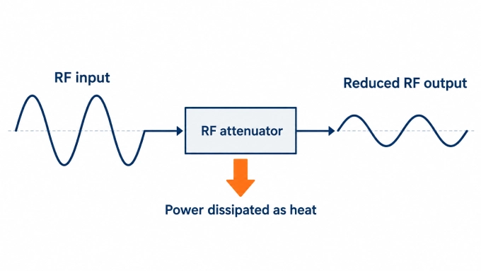
The resistance values and the way the elements are connected determine how much power is absorbed. For the same input power, greater attenuation leaves less power at the output and converts more energy into heat. Within its intended frequency range and power limits, the attenuator reduces the signal level while preserving the signal’s frequency and waveform. In practice, waveform fidelity depends on the device’s amplitude and phase response and on operation within its linear range.

What Are the Main Types of RF Attenuators?

RF attenuators can be fixed or variable. Variable models adjust attenuation either in discrete steps or continuously, giving the three main options below.

Packaging is a separate consideration. Connectorized units fit into coaxial connections, while surface-mount components are installed on circuit boards. RF attenuator ICs, also called attenuator chips, integrate the attenuation circuitry into a semiconductor device and are often supplied in surface-mount packages.

Fixed RF Attenuators

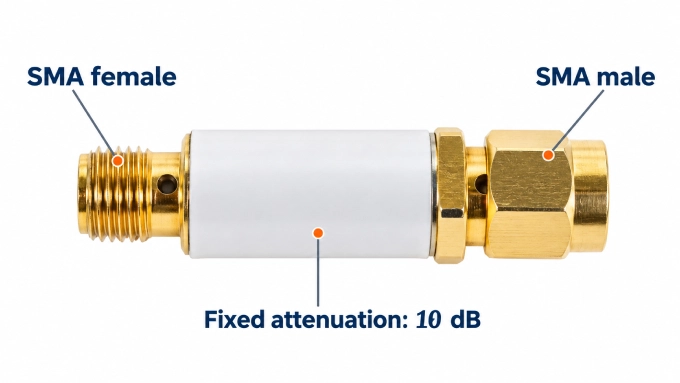
A fixed RF attenuator has one nominal attenuation value that the user cannot adjust. A 10 dB inline attenuator, for example, provides a nominal 10 dB reduction between its input and output when used under the specified conditions.

This type is appropriate when the required reduction is known and does not need to change during operation. The setting remains fixed, although the actual attenuation can still vary with frequency and temperature within the limits stated in the datasheet.

RF Step Attenuators: Manual, Digital, and Programmable Control

An RF step attenuator provides discrete attenuation settings. Its step size determines the available adjustment increments. A model with 1 dB steps, for example, might offer nominal settings of 0 dB, 1 dB, 2 dB, and so on within its adjustment range.

The settings can be selected in several ways:

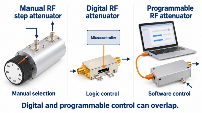
Manual RF step attenuator: A user selects discrete attenuation settings with a rotary switch, buttons, or individual switches.
Digital RF attenuator: Also called a digital step attenuator, this device uses logic signals from a microcontroller or another digital circuit to select discrete attenuation settings.
Programmable RF attenuator: Software commands control the attenuation settings, allowing remote adjustment and automated test sequences. The unit may use electronic switches or electromechanical relays.

These descriptions can overlap: a digital step attenuator can form part of a programmable unit. The word “digital” describes how the attenuation is controlled. The RF signal passes through the attenuation circuit without being converted into digital samples.

Continuously Variable RF Attenuators

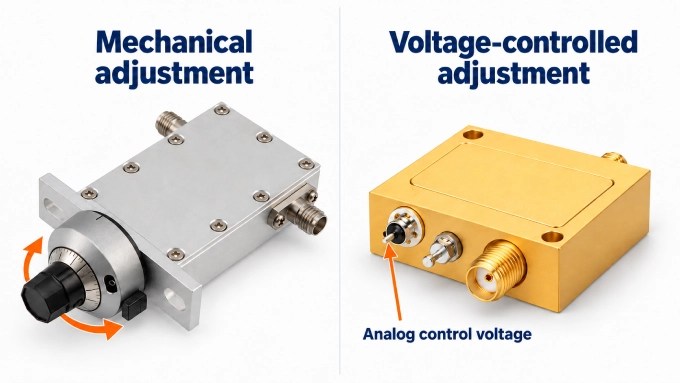
A continuously variable RF attenuator allows smooth adjustment across a defined range instead of limiting adjustment to preset steps. Mechanical models use an adjustment mechanism, often operated by a knob. A voltage-variable attenuator changes its attenuation in response to an analog control voltage.

For example, an automatic level-control circuit can monitor a signal and adjust that voltage to keep the output near a target level. The electronic control circuitry may require a DC supply. Continuous adjustment describes how the setting changes; it does not guarantee greater accuracy than a stepped design.

Which RF Attenuator Specifications Matter?

The attenuation value alone does not establish whether an RF attenuator suits a system. Its datasheet also defines the frequency range, input power, and operating conditions over which the stated performance applies.

What Do Attenuation Values in dB Mean?

Attenuation in decibels (dB) describes the ratio between input and output power. A larger positive value means a greater reduction. Because dB expresses a ratio, it does not tell you the output power unless you also know the input power.

Attenuation	Approximate output power
3 dB	Half the input power
10 dB	One-tenth
20 dB	One-hundredth
30 dB	One-thousandth

For a matched system, calculate output power using the following relationship. Both powers must use the same unit, such as watts or milliwatts:

P_{\mathrm{out}} = P_{\mathrm{in}} \times 10^{-A/10}

Here, $A$ is the attenuation in dB. The equation applies the power reduction shown in the table to any input level within the attenuator’s operating limits.

By comparison, dBm expresses an absolute power level referenced to 1 mW: 0 dBm equals 1 mW, and 30 dBm equals 1 W. Because dBm already uses a logarithmic scale, you can subtract the attenuation directly:

P_{\mathrm{out}}\,(\mathrm{dBm}) = P_{\mathrm{in}}\,(\mathrm{dBm}) - A\,(\mathrm{dB})

Voltage follows a different ratio. With equal input and output reference impedances, a 10 dB reduction leaves approximately 31.6% of the input voltage, although only 10% of the input power remains.

Frequency Range, Power Handling, and Other Specifications

The remaining specifications establish whether the attenuator can provide the required reduction under your operating conditions. Check whether quoted values are typical figures or guaranteed limits.

Specification	What it tells you
Attenuation value or range	The nominal loss of a fixed unit or the available adjustment range of a variable model.
Frequency range	The band over which specified performance applies. Both the lower and upper limits matter.
Accuracy and flatness	Accuracy describes deviation from the intended attenuation. Flatness describes variation across frequency.
Input power handling	Continuous/average and peak input limits, including any pulse-width and duty-cycle conditions. Attenuation in dB does not indicate power capacity.
Impedance	The intended system impedance, commonly 50 Ω or 75 Ω.
VSWR and return loss	The quality of the match at the ports. Lower VSWR and higher return loss indicate less reflected power.
Connectors and package	The physical interface, such as SMA or Type N, connector gender, mounting arrangement, or PCB package.
Temperature and cooling	Permitted operating temperatures and cooling conditions. Power derating specifies how allowable input power changes with operating conditions.

Adjustable models also require attention to several additional parameters:

Step size: This describes adjustment resolution. A small step size does not guarantee an equally small attenuation error.
Repeatability: This describes how closely the device reproduces the same attenuation when a setting is selected again.
Minimum insertion loss: A nominal “0 dB” setting can still introduce loss. If the other settings are specified relative to this state, total loss includes the minimum insertion loss plus the selected attenuation.
Switching and settling: Switching time characterizes the transition between settings. Settling time describes how long the output takes to remain within a stated tolerance of its final level.
Control requirements: Supply voltages, bias requirements, control-voltage ranges, logic levels, and interfaces must suit the circuit controlling the attenuator.

For semiconductor models, compression and linearity specifications describe distortion as input power increases. These are separate from damage limits: an attenuator can survive a signal level that already causes unacceptable distortion.

RF Attenuator Symbols and Circuit Diagram: Pi and T Networks

An RF attenuator symbol identifies the component’s function in a diagram, while a circuit schematic shows its internal components and connections. A block labeled with an attenuation value can represent the device without specifying its internal design.

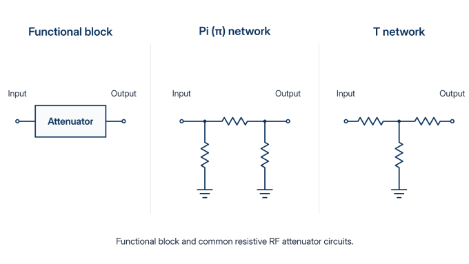
Pi and T networks are two common arrangements used in resistive attenuators:

Pi ( $π$ ) network: One series resistor connects the input and output. Two shunt resistors connect the signal path to ground, one at the input and one at the output.
T network: Two series resistors form the signal path. One shunt resistor connects their junction to ground.

A Pi attenuator is therefore one circuit implementation of an RF attenuator. In both networks, the resistor values are chosen together to provide the required attenuation and nominal port impedances. Each port presents the intended impedance when the opposite port is correctly terminated.

A well-matched pad can also improve the apparent match seen by a source. The signal is attenuated on its way to a mismatched load, and any reflected signal is attenuated again on the return path. The source sees a weaker reflection, although the load’s impedance remains unchanged.

How to Choose an RF Attenuator

The best RF attenuator for your setup provides the required loss while meeting the system’s frequency, power, and connection requirements.

Establish impedance and frequency range. Match the system impedance and cover the entire operating band.
Choose the adjustment method. Use fixed attenuation for a constant requirement, steps for selected levels, or continuous adjustment for smooth control.
Calculate the required loss. Work from the highest expected source power and the acceptable downstream operating level. Account for cable and adapter loss at the operating frequency.
Verify power handling. Check continuous and peak input limits, cooling requirements, derating, and any specified input-to-output direction.
Confirm integration. Check attenuation accuracy, connector type and gender, mounting, and control requirements. For setups requiring particular cable lengths or connector combinations, custom RF cable assemblies can connect the source, attenuator, and instrument.

Worked Example: Selecting Attenuation for a 10 W RF Source

Consider a hypothetical matched 50 Ω setup with a 10 W source (+40 dBm). The next device should receive no more than 10 mW (+10 dBm). Ignore cable and adapter loss for this calculation.

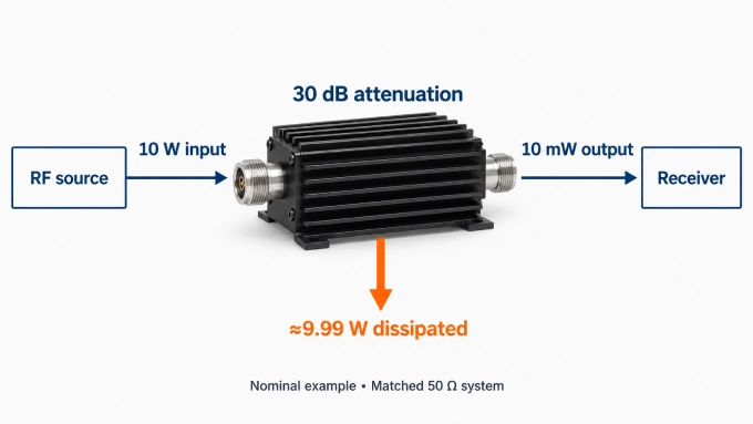
The minimum attenuation before accounting for tolerances and margin is:

A_{\min} = 40\,\mathrm{dBm} - 10\,\mathrm{dBm} = 30\,\mathrm{dB}

At nominal 30 dB attenuation, the output power is:

P_{\mathrm{out}} = 10\,\mathrm{W} \times 10^{-30/10} = 0.01\,\mathrm{W} = 10\,\mathrm{mW}

The attenuator dissipates approximately 9.99 W:

P_{\mathrm{diss}} = P_{\mathrm{in}} - P_{\mathrm{out}} = 10\,\mathrm{W} - 0.01\,\mathrm{W} = 9.99\,\mathrm{W}

A 30 dB unit rated for only 2 W cannot accept this 10 W input, even though it provides the nominal reduction required.

Also, 30 dB places the nominal output exactly at the desired limit. Lower actual attenuation or higher source power could exceed that limit. Base the final choice on the maximum expected source output and minimum guaranteed attenuation, allowing an appropriate margin. Confirm that the manufacturer’s derated input-power rating remains adequate at the operating frequency, temperature, and cooling conditions.