Can a multimeter identify whether coaxial cable is 50 Ω or 75 Ω?

No. A multimeter measures DC resistance, not the impedance experienced by a travelling RF signal. It can identify opens, shorts, and continuity problems, but it cannot determine characteristic impedance.

Does characteristic impedance change with cable length?

The characteristic impedance of a uniform cable does not depend on its length. However, cable length affects attenuation and whether test equipment can separate the cable body from connector and far-end reflections.

Does coaxial cable impedance vary with frequency?

An ideal low-loss cable has nearly constant impedance, but an actual cable may show some frequency dependence because of conductor loss, dielectric behavior, dispersion, and connector transitions. Testing should therefore reflect the intended operating range.

Should connectors be included in the impedance test?

Include them when evaluating a finished cable assembly because connector transitions affect system performance. For bulk-cable characterization, their responses should be separated through calibration, gating, de-embedding, or selection of the cable-body region.

Can capacitance alone determine characteristic impedance?

No. Total capacitance also depends on cable length, and capacitance per unit length does not uniquely determine characteristic impedance. An estimate requires additional information, such as propagation velocity for a uniform, low-loss cable, or reliable conductor geometry and dielectric properties for a construction-based calculation.

Can characteristic impedance be measured with access to only one end?

Yes, if a TDR or suitably equipped VNA provides an impedance profile with a resolvable cable-body interval before the far-end response. Access to the far-end termination is unnecessary for that interval. A short cable, unresolved connector responses, or excessive loss can make the reading inconclusive.

How to Measure The Characteristic Impedance of Coaxial Cables

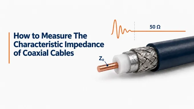
Characteristic impedance of coaxial cables can be measured through a suitable LCR, pulse-reflection testing, or a quarter-wave VNA test. These methods estimate a representative value. A time-domain reflectometer (TDR) adds an impedance profile showing cable-body impedance and local deviations. A VNA with time-domain capability can provide a similar profile, provided it supports suitable impedance processing. The procedures below focus on measuring the cable’s characteristic impedance, $Z_0$ .

If measurement equipment is unavailable, characteristic impedance can also be calculated from the conductor dimensions and dielectric constant, but this predicts the nominal design value rather than verifying the finished cable. Confirming the nominal value matters because using 75-ohm coax instead of 50-ohm in a 50 Ω path introduces impedance transitions and signal reflections.

How to Measure Characteristic Impedance with an LCR Meter

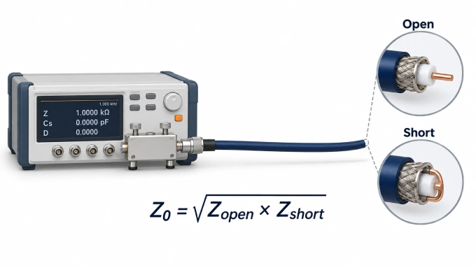
Measuring Characteristic Impedance with a LCR meter

An LCR meter can estimate the bulk characteristic impedance of a uniform coaxial cable through open- and short-circuit measurements. Use a meter with selectable test frequency and sufficient resolution for the sample’s inductance and capacitance.

Select a test frequency at which the cable is electrically short, much shorter than a wavelength, and both measurements remain within the meter’s reliable impedance range.
Connect a suitable coaxial fixture to the meter and perform the required open- and short-circuit compensation at the fixture’s DUT reference plane. Keep the cable disconnected during compensation.
Connect the near end of the cable, with its center conductor connected to the fixture’s HIGH terminal and its shield connected to LOW. Follow the fixture’s specified current and potential connections for four-terminal instruments.
Leave the far end completely open and measure total capacitance C using parallel-capacitance mode $(C_p)$ .
Create a low-inductance short between the center conductor and shield at the far end. At the same test frequency, measure total inductance L using series-inductance mode $(L_s)$ .

For sufficiently low loss, calculate characteristic impedance from the total inductance and capacitance of that same sample:

Z_0 \approx \sqrt{\frac{L}{C}}

For example, if the measurements give 2.5 µH and 1.0 nF:

Z_0 \approx \sqrt{\frac{2.5 \times 10^{-6}}{1.0 \times 10^{-9}}} = 50\ \Omega

Fixture inductance, stray capacitance, contact resistance, cable loss, and an imperfect open or short can all introduce error. The estimate is unreliable when residual fixture effects or meter uncertainty are comparable to the measured values.

Alternatively, record complex impedance in each termination state at the same frequency and use:

Z_0 = \sqrt{Z_{\mathrm{open}}Z_{\mathrm{short}}}

Use the complex impedance readings rather than resistance alone. For a uniform line, this relationship gives its potentially complex characteristic impedance at the measurement frequency, which is not automatically its nominal RF value.

How to Measure Characteristic Impedance with an Oscilloscope and Pulse Source

Find approximate characteristic impedance by minimizing the first far-end reflected pulse. Use a fast pulse source with 50 Ω output, an oscilloscope with sufficient bandwidth, a compact coaxial T connector, and low-inductance known or adjustable resistive terminations.

Connect the source output and cable’s near end to the T connector. Connect the oscilloscope to its remaining branch, using DC coupling and 50 Ω input. Keep source and scope connections short.
Leave the far end completely open. Trigger on the launched pulse and adjust the time scale to locate the first positive reflected pulse returning from the far end.
Set the pulse width shorter than the observed round-trip delay. The generator’s edge speed and scope response must distinguish launch from return; allow echoes to settle between successive pulses.
Replace the open end with known 50 Ω and 75 Ω terminations in turn, keeping other settings unchanged. Compare the first reflected pulse at the same delay. Alternatively, adjust a compact resistive termination to minimize that reflection.
Disconnect an adjustable termination from the cable and measure its resistance with a multimeter. This resistance must remain predominantly resistive over the pulse’s useful bandwidth for the estimate to be meaningful.

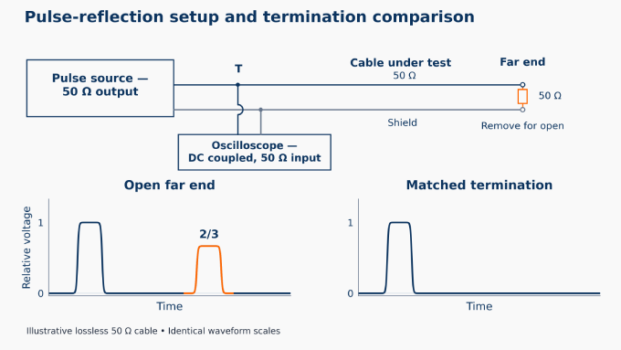
measuring characteristic impedance of coaxial cable with an Oscilloscope and Pulse Source

A matched termination absorbs the incident pulse without producing a far-end reflection, so the resistance at the minimum gives:

Z_0 \approx R_L

For a positive incident pulse, an excessively high terminating resistance produces a positive reflection; an excessively low resistance produces an inverted reflection.

An absent reflection supports a match only when the open-end test showed a clear return. Attenuation, overlapping responses, limited instrument response, and termination parasitics can make the result inconclusive.

How to Measure Characteristic Impedance with a VNA: Quarter-Wave Method

A quarter-wavelength transmission line transforms a known load according to its characteristic impedance. By measuring the cable’s input impedance at this electrical length, its characteristic impedance can be estimated. Use a sufficiently low-loss cable and a resistive load with known impedance across the sweep.

Configure a sweep starting where the cable is electrically short and extending beyond its first quarter-wave condition. If cable length $\ell$ and propagation velocity $v_p$ are known, estimate this frequency using $f_{\lambda/4} \approx v_p/(4\ell)$ .
Perform an open-short-load calibration at the cable input. Include any necessary input adapter so the calibration reference plane coincides with the cable connection.
Connect the cable to the calibrated port. Terminate the far end with a known load $(Z_L)$ .
Run the S11 sweep.Display the measurement on a Smith chart.
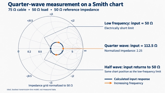
Follow the trace from its low-frequency point near $Z_L$ to the first distinct resistive-axis crossing away from that point: the quarter-wave condition. The following return toward $Z_L$ is the half-wave condition, approximately twice the frequency. If the trace barely moves, use a different known load.
Read the input impedance $(Z_{\mathrm{in}})$ at that frequency. This is the impedance looking into the terminated cable, used here to calculate $Z_0$ .
Calculate the cable’s characteristic impedance using:

Z_0 \approx \sqrt{Z_{\mathrm{in}}Z_L}

For example, if the cable is terminated with a 50 Ω load and its quarter-wave input impedance is 112.5 Ω:

Z_0 = \sqrt{112.5 \times 50} = 75\ \Omega

The method provides an estimate; its accuracy is affected by cable loss, load tolerance, connector transitions, and the correct identification of the quarter-wave point. A well-matched result at one frequency, expressed through VSWR and return loss, does not by itself establish the cable’s characteristic impedance or uniformity.

measuring characteristic impedance of coaxial cable with a VNA

How to Check Characteristic Impedance Uniformity with a TDR or VNA

A representative characteristic impedance value does not locate deviations; a suitable time-domain profile adds that information.

How to Measure Characteristic Impedance with a TDR

Measuring Characteristic Impedance with a TDR

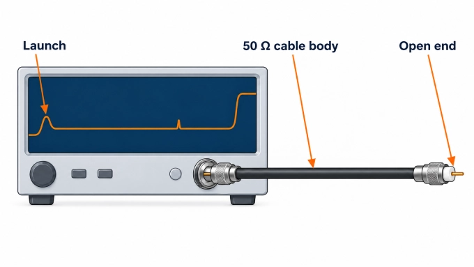
Confirm the instrument’s reference impedance. For most RF cable testing, this will be 50 Ω. Calibrate or normalize at the cable input, including any necessary adapter.
Connect the cable using the shortest appropriate adapter or transition.Leave the far end open.
Set the time span so the trace shows the launch connector, the cable body, and the far end.Choose a rise time that resolves these responses while allowing the launch to settle adequately.
Locate the stable portion of the trace after the launch response has settled and before the far-end reflection begins.
Record the average impedance of this region and note the magnitude and location of any deviations.

Measure Characteristic Impedance with a VNA Time-Domain Profile

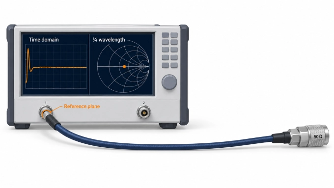
Measuring Characteristic Impedance with a VNA

Use compatible low-pass step or dedicated impedance-profile processing; a generic bandpass reflection display is insufficient.

Configure the required harmonic frequency grid, bandwidth, sweep points, and DC extrapolation before calibration.
Perform a one-port calibration at the cable input.
Connect the cable under test. Leave the far end open.
Measure S11 across a sufficiently wide frequency span.Apply the compatible step transformation and display impedance.
Enter or confirm the cable’s velocity factor if the horizontal axis displays distance.

Bandwidth controls resolution; frequency spacing limits the unaliased time range. Use this procedure for custom RF cable assemblies, including their installed connector transitions.

Interpret the Characteristic Impedance Profile

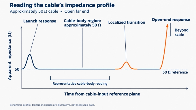
Record the average impedance of this region and note the magnitude and location of any deviations. A flat trace near 50 Ω indicates a reasonably uniform 50-ohm coaxial cable. Localized peaks or dips mark transition responses; the open end produces a large positive response.

The apparent impedance $Z$ follows:

Z = Z_{\mathrm{ref}}\frac{1+\Gamma}{1-\Gamma}

Here, $Z_{\mathrm{ref}}$ is the calibrated reference impedance, and $\Gamma$ is the normalized step-reflection coefficient. Unresolved transitions, loss, and multiple reflections can distort the apparent profile; trace shape alone does not identify a unique physical defect.

How to Calculate Coaxial Cable Characteristic Impedance from Dimensions and Dielectric Constant

When the cable geometry and dielectric properties are known, characteristic impedance can be predicted without test equipment. This method is useful for cable design, checking construction data, and estimating nominal impedance, but it does not verify the finished cable or reveal manufacturing defects.

For a uniform coaxial cable containing a homogeneous, nonmagnetic dielectric:

Z_0 \approx \frac{60}{\sqrt{\varepsilon_r}}\ln\left(\frac{D}{d}\right)

The expression assumes low-loss operation. The equivalent base-10 form is:

Z_0 \approx \frac{138}{\sqrt{\varepsilon_r}}\log_{10}\left(\frac{D}{d}\right)

Symbol

Meaning

(Z_0)

Characteristic impedance in ohms

(D)

Inner diameter of the outer conductor

(d)

Outer diameter of the center conductor

(\varepsilon_r)

Relative permittivity of the dielectric

The value of $(\varepsilon_r)$ depends on the coaxial cable dielectric material; for foamed or mixed dielectrics, use the effective relative permittivity. An unknown dielectric prevents a dependable calculation from dimensions alone.

The value of $(D)$ is not the cable or jacket diameter—it is the inside diameter of the outer conductor. Any consistent unit may be used for $(D)$ and (d) because only their ratio affects the result.

Worked Example: Calculating Approximately 50 Ω

Consider a coaxial cable with the following construction:

Inner diameter of the outer conductor: $(D = 3.5\ \mathrm{mm})$
Outer diameter of the center conductor: $(d = 1.0\ \mathrm{mm})$
Relative dielectric permittivity: $(\varepsilon_r = 2.25)$

Substituting these values into the base-10 formula gives:

Z_0 \approx \frac{138}{\sqrt{2.25}}\log_{10}\left(\frac{3.5}{1.0}\right) \approx 50\ \Omega

The calculated nominal characteristic impedance is therefore approximately 50 Ω. Increasing the ratio (D/d) raises the impedance, while increasing the dielectric permittivity $(\varepsilon_r)$ lowers it.

How to Check an Unexpected Characteristic Impedance Result

Check whether the unexpected reading changes with the setup or persists under repeat measurements. A discrepancy alone does not establish that the cable is defective.

Unstable LCR readings: Check compensation, contact repeatability, and equivalent-circuit mode. Fixture inductance, stray capacitance, contact resistance can overwhelm small readings.
Overlapping pulse responses: Compare with the open-end reference. Unresolved launch and return responses make a reflection minimum inconclusive; check pulse duration, system response, and cable delay.
Uncertain quarter-wave selection: Check the expected quarter-wave frequency against the subsequent half-wave return. Termination tolerance, connector transitions, and cable loss can obscure the crossing.
Contaminated profile region: An incorrectly positioned calibration plane, unresolved transitions, loss, or multiple reflections can contaminate the cable-body region. Check which responses the averaging interval includes.
Disagreement with a dimensional estimate: Small manufacturing variations can change the conductor spacing or effective dielectric permittivity. Check actual dimensions and dielectric assumptions; inspect for deformation, moisture, and physical damage.

Repeat after correcting suspected setup errors. Cross-check with another suitable method, accounting for frequency and loss when comparing results. Retain the measured value rather than rounding it to 50 Ω or 75 Ω.

The reported value should therefore identify what was measured:

Method, test frequency or bandwidth, and relevant instrument settings.
Sample length, reference plane, fixtures, and far-end termination.
Representative cable-body value, evaluated region, local deviations, and measurement uncertainty.

There is no universal acceptable tolerance. The limit should come from the cable specification and the system’s reflection budget. Both the average impedance and the magnitude of local deviations should be considered. Apply the specification’s stated measurement conditions when making that comparison.