Is Transfer Impedance the Same for Ingress and Egress?

Under linear, passive, reciprocal conditions, the same transfer-impedance parameter describes coupling in either direction when reference directions and normalization are applied consistently. Reversing the test, however, does not guarantee identical terminal voltages. Source and load impedances, shield-current distribution, propagation, and the selected near- or far-end response can differ between configurations.

Can Good Return Loss and Insertion Loss Demonstrate Low Transfer Impedance?

No. Return loss and insertion loss characterize transmission through the intended coaxial signal path. Transfer impedance characterizes coupling between the shield’s external and internal circuits. A cable or assembly can meet transmission-loss and matching limits while failing its shielding requirement, so low transfer impedance must be demonstrated with an applicable shield-coupling measurement.

Is Magnitude-Only Transfer-Impedance Data Enough for Transient Simulation?

No. A magnitude curve omits the phase needed to reconstruct a unique time-domain response. Transient analysis normally requires the complex surface transfer impedance over sufficient bandwidth and frequency resolution, or a validated causal model fitted to equivalent data. The model must also represent the shield current, cable topology, propagation, and source and load terminations.

Coaxial Cable Transfer Impedance: What It Means for RF Shielding Performance

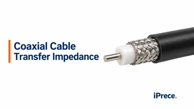
Coaxial cable transfer impedance is a parameter used to quantify shield coupling performance in coaxial and other shielded cables. Because it varies with frequency, shield construction, and test configuration, a single value or generic shielding claim can be misleading. This article explains how to read $Z_T(f)$ , how different shield constructions shape the response, how transfer impedance is measured, and how to translate valid data into an application-specific coupling limit.

What Does Coaxial Cable Transfer Impedance Quantify?

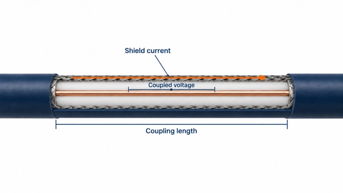
Coaxial cable transfer impedance, $Z_T$ , quantifies how much longitudinal voltage is coupled into the cable’s internal circuit by current flowing in the external shield circuit. For a uniform cable section, its local definition is:

Z_T(f)=\frac{1}{I_s(f)}\frac{\mathrm{d}V_{\mathrm{ind}}(f)}{\mathrm{d}z}

where:

$Z_T(f)$ is the complex surface transfer impedance in Ω/m
$I_s(f)$ is the shield current in the external circuit
$\mathrm{d}V_{\mathrm{ind}}/\mathrm{d}z$ is the induced longitudinal voltage per unit length in the internal circuit

A lower $Z_T$ therefore indicates less current-driven coupling through the shield under comparable conditions. Because transfer impedance is complex, it contains both magnitude and phase information. Datasheets commonly report only $Z_T$ , often in mΩ/m.

Transfer impedance is not the cable’s characteristic impedance. A 50 Ω or 75 Ω rating describes the voltage-to-current relationship of the intended transmission mode; $Z_T$ describes coupling across the shield. Values specified in Ω/m also apply to distributed cable, whereas a connector or localized shield discontinuity may have a lumped transfer impedance stated in Ω.

How Do You Calculate the Voltage Coupled Through the Shield?

For a uniform, electrically short cable section carrying approximately constant shield current, the total induced source voltage is:

V_{\mathrm{ind}}(f)\approx Z_T(f)I_s(f)L

Suppose radio frequency interference produces a 20 mA shield current at 1 MHz along a 0.5 m cable section whose transfer impedance is:

Z_T=(3+j4)\ \mathrm{m\Omega/m}

The induced source voltage is:

V_{\mathrm{ind}}=(3+j4)\times10^{-3}\times20\times10^{-3}\times0.5

V_{\mathrm{ind}}=(30+j40)\ \mathrm{\mu V}

and its magnitude is:

\left|V_{\mathrm{ind}}\right|=50\ \mathrm{\mu V}

That 50 µV is the distributed source voltage coupled into the internal circuit—not automatically the voltage appearing at one receiver. In this simplified example only, the cable section is electrically short and the internal circuit has equal 50 Ω terminations at both ends. Under those assumptions, the induced voltage divides equally, giving approximately:

\left|V_{\mathrm{load}}\right|\approx\frac{\left|V_{\mathrm{ind}}\right|}{2}=25\ \mathrm{\mu V}

Once the cable is no longer electrically short, propagation delay, shield-current variation, source and load impedances, and the phase of coupling along the cable determine how the distributed contributions combine. A uniform external field also does not guarantee uniform shield current.

Why Does Transfer Impedance Vary with Frequency and Shield Construction?

Transfer impedance varies because the mechanisms carrying energy through a shield change with frequency. For many cable shields, a useful engineering model is:

Z_T(f)\approx Z_d(f)+j\omega L_T(f)

Here, $Z_d$ represents conductor resistance and electromagnetic diffusion through the shield material, while $L_T$ represents the net inductive coupling associated with apertures, seams, and the geometry of the current paths. This is a conceptual decomposition rather than a universal equivalent circuit.

At sufficiently low frequencies, where skin depth is large relative to the effective shield thickness, current penetrates much of the conducting cross-section. The transfer impedance then approaches a resistance-dominated value related to shield conductivity, metal area, and electrical contact between shield elements.

As frequency rises and skin depth decreases, diffusion through a continuous conductor is reduced. A homogeneous solid shield may therefore show a declining $Z_T$ . In a braid or another discontinuous shield, however, magnetic flux can also couple through apertures and between the interwoven current paths. Once the inductive term dominates and L_T is approximately constant over a limited range:

\left|Z_T\right|\approx\omega L_T

The magnitude then rises approximately in proportion to frequency, corresponding to about 20 dB per decade. Practical curves may show a minimum where the declining diffusion contribution gives way to inductive coupling. The position and slope of that transition are not universal because $L_T$ itself can vary with geometry and frequency.

Here’s how shield construction and Mechanisms affecting $Z_T(f)$ are related:

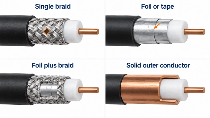
Single braid: Conductivity and total wire area influence the low-frequency resistance. At higher frequencies, carrier count, wire diameter, weave angle, crossover geometry, and aperture size affect inductive coupling. Two braids with equal optical coverage can therefore have different transfer-impedance curves.
Foil or tape: Metal thickness controls diffusion through the conductive layer, while seam geometry, overlap, drain-wire contact, and continuity along the cable influence longitudinal current flow and aperture coupling. Near-complete visual coverage does not establish low transfer impedance if the seam or contact path is poor.
Foil-plus-braid or multiple shields: Performance depends on the individual layers and on how they interact. Electrical contact or isolation between layers, interlayer spacing, seam orientation, and current sharing can change the resulting response. The labels “double shield” or “foil plus braid” are therefore insufficient specifications by themselves.
Continuous solid outer conductor: With no braid apertures or longitudinal foil seam, the bulk response is primarily diffusion-dominated and provides a useful reference case. Joints, connector interfaces, and other discontinuities can still determine the shielding performance of the finished assembly.

For custom RF cable assemblies, request frequency-dependent data for the specified shield construction and identify whether it covers bulk cable or the connectorized assembly.

How Does Transfer Impedance Differ from Shielding Effectiveness?

Transfer impedance, shielding effectiveness, and screening attenuation all describe shield behavior, but they are not interchangeable specifications.

Metric	What is measured	Units and interpretation	Required reference conditions
Transfer impedance, Z_T	Longitudinal voltage coupled into the internal circuit per unit shield current and cable length	Ω/m, commonly mΩ/m; lower is better	Frequency, test method, active length, circuit configuration, and specimen construction
Shielding effectiveness, SE	Reduction in coupled field, voltage, or power produced by adding the shield	dB; higher is better	Excitation type, field impedance, geometry, terminations, cable length, and shielded/unshielded reference measurements
Screening attenuation, a_S	Power transmitted through the shield in a defined cable test configuration	dB; higher is better	Standardized fixture, launched mode, reference power, specimen length, terminations, and valid frequency range

There is no configuration-independent conversion from Ω/m to dB. A shielding-effectiveness result depends on the specified excitation, reference response, and receiving circuit—not on $Z_T$ alone.

Transfer impedance does not necessarily describe every coupling mechanism. IEC 62153-4-3 determines the magnetic component of surface transfer impedance. Capacitive coupling is represented separately by transfer admittance, $Y_T$ , expressed in S/m and measured under IEC 62153-4-8. For most well-screened coaxial cables this contribution may be negligible, but it can become relevant when electric fields couple through openings in a loose single braid. In such cases, $Z_T$ alone does not completely characterize the shield.

How Should Coaxial Cable Transfer Impedance Be Measured?

Choose the measurement method for the intended test object: bulk cable, a connector transition, or a complete assembly.

Bulk-cable surface transfer impedance: IEC 62153-4-3:2013+AMD1:2024, using a triaxial fixture formed by the cable under test and a surrounding conductive tube or equivalent outer conductor
Alternative excitation of bulk cable: IEC 62153-4-6:2017 line-injection method, applicable from a few kilohertz to above 1 GHz when its configuration and validity requirements are met
Connectors, cable-to-connector transitions, and assemblies: IEC 62153-4-7:2021+AMD1:2025 tube-in-tube method; IEC 62153-4-15:2021+AMD1:2024 provides triaxial-cell procedures for connectors, assemblies, and other components
Screening attenuation: IEC 62153-4-4:2015 triaxial method; report $a_S$ rather than extending a transfer-impedance extraction beyond its valid range

The usable upper frequency for transfer-impedance extraction is not universally 100 MHz. Under IEC 62153-4-3, it depends on the selected triaxial test configuration, coupling length, propagation velocities, and termination conditions. The approximately 30 MHz range for a 1 m specimen and 100 MHz range for a 0.3 m specimen are configuration-specific examples under that method—not general limits for all transfer-impedance measurements. Other methods, configurations, and specimen lengths have different valid frequency ranges.

Set Up the Measurement and Extract $Z_T$

In a triaxial measurement, the center conductor and inside surface of the cable shield form the inner circuit. The outside surface of that shield and the inner wall of the surrounding conductive tube form the outer circuit. For an ingress-oriented configuration, the generator drives the outer circuit so that a controlled current flows along the shield and returns through the tube; the receiver measures the voltage coupled into the terminated inner circuit.

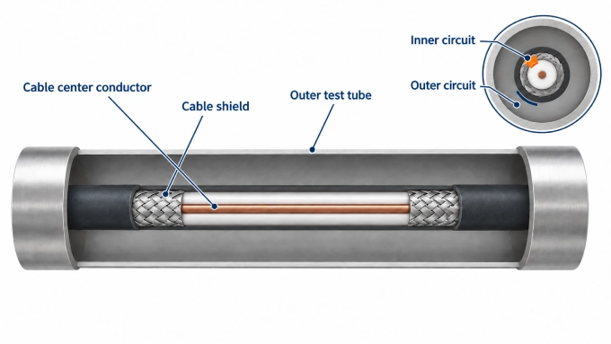
Establish the active coupling length. Use the shield boundaries within the fixture, not the overall cut length.
Prepare and install the specimen. Make the shield bonds, fixture connections, shorts, and terminating loads required by the selected standard configuration. Avoid altering the braid geometry, foil overlap, or layer contact during preparation. For assembly tests, document connector mating, torque, adapters, and the transition included within the measurement region.
Set and calibrate the reference planes. Calibrate the VNA—or the generator and selective receiver—to the accessible fixture planes. Account for cables and adapters using the correction or de-embedding procedure appropriate to the fixture. Confirm the inner- and outer-circuit impedances used in the calculation and control unintended ground loops, particularly at low frequencies.
Verify the usable measurement range. Establish residual fixture coupling and receiver noise before testing the specimen. Check linearity by changing the source level and confirming the expected proportional response without receiver compression. The reported band must remain within both the fixture’s valid propagation range and the available dynamic range.
Acquire the coupling response. Sweep the required frequencies using documented source power, bandwidth, averaging, and termination conditions. Determine the shield current from the quantities and circuit model prescribed by the selected method; do not assume that the VNA source setting equals the current flowing on the shield.
Calculate transfer impedance. Apply the configuration-specific conversion to the measured response, including the relevant circuit impedances, near- or far-end termination factor, fixture correction, and normalization by active coupling length. Raw $S_{21}$ is a transmission ratio, not transfer impedance, and no single conversion equation applies to every triaxial configuration.
Preserve reproducibility. Report the specimen construction and condition, active length, fixture and standard edition, topology, termination values, calibration procedure, reference planes, instrument settings, environmental conditions, valid bandwidth, measurement floor, and estimated uncertainty. Repeat installation when connection repeatability could materially affect the result.

How Should You Interpret Transfer-Impedance Data and Set Requirements?

Interpretation should begin only after confirming that the plotted response represents the intended specimen over the valid measurement band. Once validated, compare it with a frequency-dependent requirement derived from the application’s coupling budget—not with a generic transfer-impedance threshold.

Separate Shield Behavior from Measurement Artifacts

For logarithmic plots, confirm the stated reference quantity before comparing traces.

If the specimen response cannot be distinguished from receiver noise and residual fixture coupling, report it as unresolved rather than as an exact transfer-impedance value. Quote an upper bound only when the measurement procedure establishes one.

Observation	Controlled check	What the result can establish
Narrow peak or minimum	Reconnect the specimen and repeat the sweep	Whether the feature is sensitive to contacts, bonds, or fixture assembly
Feature at the upper end of the sweep	Repeat with a shorter coupling length or another valid configuration	Whether propagation and the method’s frequency limit are influencing the curve
Unexpected offset between specimens	Repeat the complete preparation and installation process	Whether specimen variation exceeds connection repeatability

Finite-length measurements can contain resonances caused by mismatch or different propagation velocities in the inner and outer circuits. Check these effects before assigning a material cause. Repeatable deterioration after those checks warrants investigation for coaxial cable shielding failure, but the curve alone cannot identify the defect.

Compare Candidates Against a Frequency-Dependent Acceptance Limit

Compare equivalent test objects using compatible methods, conditions, normalization, and valid frequency ranges. Identify whether each result is a typical curve, a guaranteed limit, or a measurement from a stated sample population.

Within the assumptions of the earlier short-section model, the coupling budget gives:

\left|Z_{T,\mathrm{limit}}(f)\right| \leq \frac{\left|V_{\mathrm{ind,max}}(f)\right|} {\left|I_s(f)\right|L}

The allowable induced voltage must be established from the receiver or circuit limit after accounting for its terminations. Apply the relationship across the relevant shield-current spectrum rather than at one convenient frequency. If measurement uncertainty is significant near the limit, acceptance should follow a declared decision rule—commonly requiring the upper uncertainty bound to remain below the limit.

Do not compare a lumped connector value in Ω directly with cable data in Ω/m, or normalize it by an arbitrary cable length.