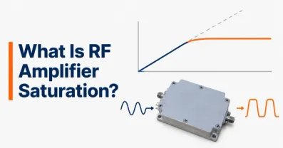
What Is RF Amplifier Power Back-Off? IBO, OBO, and PAPR


Power backoff is the reduction in an RF power amplifier's operating power relative to a defined reference level, typically its saturation power or 1 dB compression point. Engineers use back-off to limit nonlinear distortion, preserve modulation quality, and prevent signal peaks from driving the amplifier too far into compression.
The difficulty is finding the right amount. Excessive back-off wastes available output power and often reduces efficiency. Insufficient back-off can increase intermodulation distortion, error vector magnitude (EVM), and adjacent-channel emissions.
The practical question is therefore not simply how far below saturation an amplifier should operate, but what is the highest average output power that still meets the waveform's linearity, efficiency, and reliability requirements?
Understanding Power Backoff in an RF Amplifier
RF amplifier power back-off describes the difference between a reference power level and the amplifier's actual operating power, expressed in decibels.
An amplifier normally produces approximately proportional output power over its small-signal operating region. At higher drive levels, gain compression becomes significant, eventually approaching the device's saturated output power .
Operating below that region provides headroom for signal peaks.
Two reference levels are commonly used:
Saturation power (Psat): The output power approached near saturation, according to the manufacturer's measurement definition.
1 dB compression point (P1dB): The CW operating point where gain has decreased by 1 dB relative to its small-signal value.
These references are not interchangeable. An amplifier may have an output P1dB of +37 dBm and a Psat of +40 dBm.
For the same average output power, back-off relative to Psat is therefore 3 dB greater than back-off relative to P1dB. Always specify the reference when quoting a back-off value. A statement such as “the amplifier operates with 8 dB back-off” is incomplete without identifying the reference and whether the value applies to input, average output, or signal peaks.
What Are the Differences Between IBO, OBO, and Peak Back-Off?
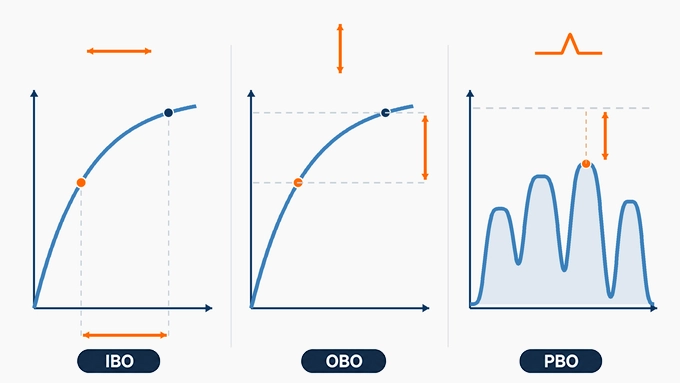
Input back-off, output back-off, and peak back-off describe different operating margins.
Parameter | Reference | Operating Quantity | Main Purpose |
Input Back-Off (IBO) | Input power at saturation or compression | Average input power | Controls amplifier drive |
Output Back-Off (OBO) | Output power at saturation or compression | Average output power | Defines available output headroom |
Peak Back-Off (PBO) | Output saturation or compression reference | Peak envelope output power | Evaluates peak-power headroom |
Input Back-Off (IBO)
Input back-off measures how far the average input drive is below a specified input reference.
Using input power at saturation:
Both powers are expressed in dBm, producing an IBO result in dB. IBO is useful when configuring the preceding driver stage or signal generator.
Output Back-Off (OBO)
Output back-off measures how far the amplifier's average output power is below its reference output capability.
Using saturated output power:
OBO describes how much nominal output-power capability remains unused at the average operating point. It is particularly useful when comparing amplifier operation with efficiency curves.
Peak Back-Off (PBO)
Peak back-off measures the margin between the reference output power and the waveform's peak envelope power.
For a desired undistorted output waveform:
This relationship is essential for amplifiers handling signals with varying envelopes.
A PA can have substantial average output back-off while still operating close to compression during its highest peaks.
Important: A peak below the measured CW Psat is not necessarily sufficiently linear. Distortion can become unacceptable well before saturation.
How Do You Calculate Input and Output Power Back-Off?
Back-off calculations are straightforward when all power values use the same reference convention.
The challenge is ensuring that input saturation, output saturation, and average operating powers correspond to the same amplifier, frequency, bias, and load conditions.
Worked Example: IBO, OBO, and Peak Back-Off
Consider a hypothetical RF power amplifier with the following measured or assumed characteristics:
Parameter | Value |
Small-signal gain | 20 dB |
Input power at saturation | +22 dBm |
Saturated output power | +40 dBm |
Output P1dB | +37 dBm |
Average input power | +8 dBm |
Average output power | +28 dBm |
Desired output waveform PAPR | 8 dB |
Step 1: Calculate input back-off.
Step 2: Calculate output back-off relative to saturation.
Step 3: Determine the desired peak output power.
Step 4: Calculate peak back-off.
The intended peaks are 4 dB below Psat but only 1 dB below the CW output P1dB.
That 1 dB margin is not proof that the waveform meets its EVM or ACLR requirements. Those specifications must be measured with the actual modulation.
Why Are IBO and OBO Different?
IBO and OBO are not necessarily equal because amplifier gain changes with drive level.
In this example:
Gain at the average operating point: (28-8=20) dB
Gain at saturation: (40-22=18) dB
The relationship is:
Therefore:
The 2 dB difference is consistent with the assumed reduction in gain near saturation.
Using IBO and OBO interchangeably without accounting for compression can lead to incorrect operating-point calculations.
How Does PAPR Affect Power Back-Off in RF Amplifiers?
Peak-to-average power ratio (PAPR) describes the relationship between the maximum envelope power and average RF power.
In dB:
Signals with approximately constant envelopes generally require less peak headroom than signals with large envelope variations.
OFDM, multicarrier, and certain higher-order modulated signals can exhibit substantial PAPR.
Why Average Power Alone Is Misleading
Consider two signals transmitted through the same amplifier at +28 dBm average output power.
Characteristic | Signal A | Signal B |
Average output | +28 dBm | +28 dBm |
Desired PAPR | 3 dB | 10 dB |
Desired peak output | +31 dBm | +38 dBm |
Peak margin to +40 dBm Psat | 9 dB | 2 dB |
Although average output power is identical, Signal B places much greater demands on the amplifier's peak-power capability. This is why a back-off value that works for one waveform may fail for another.
PAPR Statistics and CCDF
For noise-like modulated signals, the highest observed peak depends on waveform length, filtering, oversampling, and signal statistics.
A Complementary Cumulative Distribution Function (CCDF) describes the probability that instantaneous envelope power exceeds a given level relative to its average. For example, a CCDF value of (10^{-4}) indicates that approximately 0.01% of the evaluated samples exceed the corresponding power level.
A CCDF-based PAPR is meaningful only when its probability threshold and measurement conditions are specified. Engineers should characterize the waveform before the amplifier, then compare the intended envelope with the actual output response.
A compressed amplifier may reduce measured output PAPR by clipping peaks. A lower output PAPR caused by compression is not evidence that the amplifier has sufficient headroom.
How Does Power Back-Off Affect Amplifier Linearity and Efficiency?
Increasing back-off generally reduces nonlinear distortion, but it also reduces the amplifier's usable average output power. The reason is that transistor efficiency is usually dependent on output level.
Many conventional power amplifier architectures achieve their highest efficiency near large-signal operation. As average output power decreases, DC consumption may not fall proportionally. Consequently, power-added efficiency (PAE) often decreases.
Power Back-Off and Linearity
At lower average drive levels, an amplifier generally experiences less gain compression and reduced nonlinear distortion.
This can improve:
EVM and modulation accuracy
Adjacent Channel Leakage Ratio (ACLR)
Intermodulation distortion performance
Spectral mask compliance
However, back-off cannot guarantee a particular distortion specification.
Some amplifiers exhibit substantial AM-PM distortion or memory effects even when average power is well below P1dB. The relationship between output power and distortion must therefore be characterized under the intended waveform.
Power Backoff vs. Efficiency
Power-added efficiency is defined as:
All powers in this equation must be expressed in watts.
Suppose the amplifier in the previous example delivers +28 dBm average output power with +8 dBm average input power.
These correspond to approximately 0.631 W and 0.0063 W.
If the measured DC consumption is 3.67 W:
This value is illustrative. The actual efficiency must be measured at the operating frequency, output power, waveform, bias, and temperature.
A 12 dB OBO does not imply any universal PAE value. Different amplifier architectures can exhibit substantially different efficiencies at the same output back-off.
How Should RF Engineers Determine the Required Power Back-Off?
The required back-off should be established by testing the actual waveform against the system's linearity and efficiency requirements.
A formula based only on Psat and PAPR can provide an initial operating estimate, but it cannot replace waveform-dependent measurements.
Step 1: Define the Required Signal Quality
Start with the application's measurable acceptance criteria.
These may include:
Maximum EVM
Minimum ACLR, expressed as a positive ratio, or maximum adjacent-channel power in dBc
Spectral emission limits
Minimum delivered average output power
Maximum DC consumption and device temperature
Use the measurement bandwidths, filtering, and definitions associated with the applicable communication standard.
Step 2: Characterize the Intended Waveform
Measure average power and PAPR using a representative waveform.
Record the waveform bandwidth, modulation, CCDF characteristics, and any crest factor reduction already applied. Do not select a back-off value using a generic PAPR estimate if the actual waveform is available.
Step 3: Establish an Initial Output-Power Limit
Select a suitable output reference, such as measured Psat or OP1dB, and document it.
For an initial estimate:
Where () is an additional engineering margin.
The peak limit and margin must be supported by amplifier characterization. They are not universal constants.
For example, if the selected provisional peak limit is +37 dBm, the waveform PAPR is 8 dB, and an additional 1 dB margin is required:
This establishes a starting point, not a guaranteed linear operating limit.
Step 4: Sweep Output Power and Measure Distortion
Increase average output power in controlled increments while measuring EVM, ACLR, input power, DC consumption, and temperature.
Consider the following hypothetical results for a linearized RF power amplifier:
Average Output | OBO from +40 dBm Psat | EVM | Adjacent Power | PAE |
+26 dBm | 14 dB | 1.5% | −49 dBc | 13% |
+28 dBm | 12 dB | 2.1% | −46 dBc | 17% |
+30 dBm | 10 dB | 3.4% | −41 dBc | 22% |
Suppose the application requires:
EVM no greater than 2.5%
Adjacent-channel power no greater than −45 dBc
The +30 dBm operating point fails both requirements. The +26 dBm and +28 dBm points meet the stated nominal limits.
Of those tested points, +28 dBm provides the greater output power and higher PAE while meeting the stated requirements. The provisional choice is therefore +28 dBm, corresponding to 12 dB output back-off relative to Psat.
Step 5: Apply Operating Margins
Before approving that operating point, repeat the measurements across the required frequency band, supply range, temperature range, and load conditions.
Account for measurement uncertainty, device variation, aging where relevant, and the specified production acceptance rule. If the +28 dBm result cannot maintain sufficient margin under those conditions, more back-off or additional linearization may be necessary.
The best operating point is the highest efficient output level that satisfies all requirements with appropriate margin—not simply the highest power measured during a laboratory sweep.
How Can RF Amplifier Efficiency Be Improved at Back-Off?
Reducing back-off improves average output-power utilization, provided the amplifier still meets its linearity requirements. Several techniques help balance efficiency and distortion.
For a more detailed explanation of compression, EVM, and intermodulation mechanisms, see RF amplifier linearity.
Digital Predistortion (DPD)
DPD compensates for amplifier nonlinearity, reducing EVM and spectral regrowth while enabling higher average output power. Its effectiveness depends on model accuracy, feedback quality, bandwidth, and memory effects, without eliminating physical peak-power limits.
Doherty Power Amplifiers
Doherty amplifiers use carrier and peaking paths with load modulation to improve efficiency under backed-off operation, particularly for high-PAPR signals. DPD is often required to maintain linearity.
Crest Factor Reduction (CFR)
CFR reduces signal peaks and PAPR, potentially allowing higher average output power. For example, reducing PAPR from 10 dB to 7 dB can provide 3 dB of additional average-power headroom at the same peak limit. However, waveform modifications may increase EVM and spectral emissions.
Envelope Tracking and Adaptive Bias
Envelope tracking adjusts supply voltage to the signal envelope, while adaptive bias optimizes operating conditions to improve efficiency. Both require careful management of control bandwidth, timing, noise, and linearity.
Power backoff establishes the operating margin between an RF amplifier's actual power and a defined compression or saturation reference. IBO describes input-drive reduction, OBO describes average output-power reduction, and PBO describes the remaining margin for signal peaks. PAPR explains why average power alone cannot establish whether a modulated signal will remain sufficiently linear. The appropriate RF amplifier power back-off is the smallest amount that reliably satisfies the application's linearity, spectral, thermal, and operating constraints. To determine it, measure the intended waveform, characterize distortion and efficiency across output power, and validate the chosen operating point under representative conditions. Techniques such as DPD, Doherty amplification, and CFR can then be evaluated to recover efficiency without sacrificing required signal quality.
FAQ
Discussion (0)
Be the first to comment.