What Is Atmospheric Attenuation? Calculation Formula & Chart

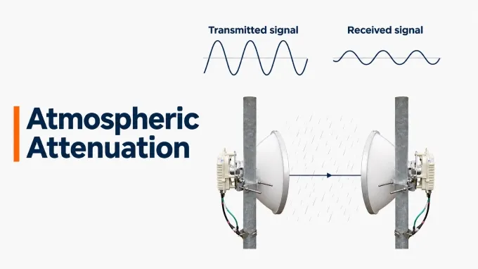
Atmospheric attenuation is the reduction in RF signal power caused by interactions with gases and particles as a radio wave travels through the atmosphere. The amount of loss depends on the signal’s frequency, atmospheric conditions, and the length and route of its path through the air.
This effect matters in terrestrial microwave links, satellite communications, and RF radar systems because it reduces the useful signal power reaching the receiver. The atmosphere can introduce this loss in clear weather as well as during rain or fog. This discussion focuses on attenuation at microwave and millimeter-wave frequencies.
How Does Atmospheric Attenuation Work?
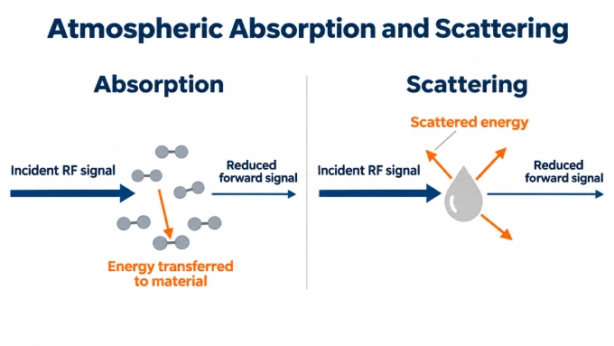
The atmosphere weakens an RF signal through absorption and scattering. These mechanisms can occur together, and their effects accumulate along the propagation path. The total loss depends on the conditions encountered and the distance the signal travels through each region.
Atmospheric Absorption
During atmospheric absorption, the wave’s electric or magnetic field interacts with molecules in the medium and transfers some of its energy to them. Collisions between molecules redistribute the absorbed energy, ultimately converting it into heat. The wave continues to propagate, but it carries less power after passing through the absorbing region.
Atmospheric Scattering
Scattering occurs when particles interact with the wave and redirect part of its energy into other directions. The scattered energy remains electromagnetic radiation, but some of it no longer travels toward the intended receiver. Particles can scatter energy forward, backward, or sideways, depending on their properties and size relative to the signal’s wavelength.
What Causes RF Atmospheric Attenuation?
The main contributors to atmospheric attenuation in microwave and millimeter-wave systems are oxygen, water vapor, rain, and the liquid droplets in clouds and fog.
Oxygen (Gas): A principal contributor to gaseous absorption. Its effect depends on frequency and the atmospheric state.
Water vapor (Gas): Contributes to gaseous absorption. Its concentration varies with atmospheric conditions and differs from the liquid water content of clouds or rain.
Rain: Produces absorption and scattering. Rain rate, drop characteristics, frequency, and polarization influence the loss.
Liquid-water clouds and fog: Suspended liquid droplets attenuate the signal. Liquid water content, temperature, frequency, and the distance traveled through the droplets affect the loss. ITU-R P.840-9, Annex 1.
Humidity alone does not establish how much liquid water lies along a path. High humidity, fog, and rainfall therefore cannot be treated as interchangeable conditions when estimating attenuation.
Humidity, temperature, and pressure modify these contributions; they are environmental parameters, not additional attenuation mechanisms. ITU-R addresses gaseous attenuation, rain attenuation, and cloud or fog attenuation through separate recommendations because they require different physical models and inputs.
When and How Should RF Engineers Account for Atmospheric Attenuation?
Atmospheric attenuation consumes link margin and can reduce communication availability or radar detection performance. Engineers should evaluate its importance against the expected operating conditions and the system’s required performance.
When Does Atmospheric Attenuation Become Significant?
Atmospheric attenuation becomes significant when the loss threatens the received power or signal-to-noise ratio required for reliable operation. Explicit evaluation is particularly important when:
The operating frequency is susceptible to gaseous absorption or substantial weather-related loss.
A long terrestrial path exposes the signal to atmospheric losses over an extended distance.
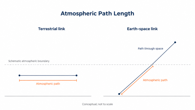
An Earth–space link operates at low elevation, increasing the distance traveled through the atmosphere.
The system has limited margin or must maintain high availability despite adverse weather.
Frequency alone does not determine significance. A short link with ample margin may tolerate conditions that require explicit allowances on a longer or more demanding link. The decision should follow the actual path, expected atmospheric conditions, and allowable performance degradation.
How Atmospheric Attenuation Enters an RF Link Budget
Include atmospheric attenuation as a separate loss term in the received-power budget:
Here, and are transmitted and received powers in dBm, while and are antenna gains in dBi. All loss terms are in dB; represents atmospheric attenuation.
Loss or effect | Treatment |
Free space path loss | Geometric spreading, represented by . |
Refraction and scintillation | Changes in propagation direction or received level; evaluate with an appropriate propagation model. |
Interference and noise | Evaluate interference and total system noise, including noise generated inside the receiver, when calculating SNR or SINR. |
Feeder and hardware losses | Include coaxial cable signal loss and other hardware insertion losses in |
For Earth–space links, atmospheric absorption is accompanied by thermal emission that contributes to antenna noise temperature. Assess this noise contribution alongside the reduction in received signal power when estimating SNR. ITU-R P.618-14, §3.
For reciprocal radar paths using the same frequency, atmospheric loss occurs on both the outward and return legs. The round-trip atmospheric loss is twice the one-way value.
Depending on the application, engineers can select a suitable transmission window, shorten hops, reserve fade margin, adapt modulation or coding, or use diversity. These measures should support the required performance and availability.
Atmospheric Attenuation Coefficient: Meaning, Units, and Formula
The atmospheric attenuation coefficient describes how rapidly atmospheric loss accumulates with distance. RF engineers commonly express it as specific attenuation, , in dB/km. Path attenuation, , is the accumulated loss along a defined path, expressed in dB.
When atmospheric conditions vary along the path, you can calculate the accumulated attenuation. The atmospheric attenuation formula is:
Symbol | Meaning | Unit |
Specific attenuation at position s | dB/km | |
Accumulated atmospheric attenuation | dB | |
Distance along the propagation path | km | |
Length of the path being assessed | km |
The integral adds the local losses along the route. In practice, the path can be divided into regions with approximately uniform conditions, and the losses from those regions can be added.
For a homogeneous path, the relevant atmospheric conditions remain constant, so specific attenuation has one value at the chosen frequency. The expression simplifies to:
For gaseous attenuation, combine the dry-air and water-vapor contributions:
Evaluate both contributions at the same frequency, temperature, pressure, and water-vapor density. These inputs determine the gaseous coefficient, so a value calculated for one atmospheric state may not represent another. Using a single coefficient for the entire path assumes that its inputs adequately represent conditions throughout that path.
Atmospheric Attenuation vs Frequency
For a fixed atmospheric state, gaseous attenuation varies with frequency through absorption peaks and lower-loss transmission windows. It does not follow a steadily increasing curve: a higher frequency can sometimes experience less gaseous loss than a lower one.
Specific Gaseous Attenuation vs Frequency
The chart shows specific gaseous attenuation due to dry air, water vapor, and their combined contribution at a defined atmospheric state. It helps identify absorption peaks and relatively low-loss transmission windows. Rain and cloud attenuation are not included. Use the component curves to identify which contribution dominates a particular frequency band.
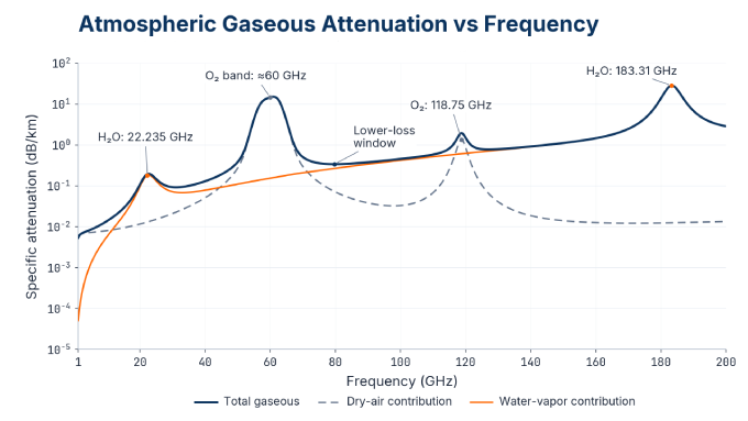
Atmospheric conditions: 1,013.25 hPa pressure, 15°C temperature, and 7.5 g/m³ water-vapor density.
Water vapor produces absorption features near 22.235 GHz and 183.31 GHz. The dry-air contribution contains a broad oxygen absorption band around 60 GHz and another oxygen feature near 118.75 GHz. These features identify regions where molecular absorption becomes particularly strong.
The logarithmic vertical axis allows large differences in specific attenuation to remain readable. Equally spaced ticks represent multiplicative changes: the interval from 0.01 to 0.1 dB/km occupies the same vertical distance as 0.1 to 1 dB/km.
Transmission windows lie in the lower regions between absorption features. They indicate relatively favorable frequencies for propagation through the specified atmosphere, but they still have finite gaseous loss. Their relevance to a link depends on its path length and allowable attenuation. The chart does not establish total weather-related loss; rain and suspended droplets require separately defined conditions.
Atmospheric Attenuation vs Wavelength
Shorter wavelengths correspond to higher frequencies. Using the free-space approximation, the relationship is:
Here, is wavelength, is frequency, and is the speed of light in vacuum. With frequency in hertz and in meters per second, wavelength is obtained in meters.
Frequency | Approximate wavelength |
10 GHz | 30 mm |
22.235 GHz | 13.5 mm |
60 GHz | 5 mm |
183.31 GHz | 1.64 mm |
Expressing the spectrum against increasing wavelength would reverse the horizontal order of its features. Each corresponding frequency–wavelength pair would retain the same attenuation value under the specified atmospheric conditions. The conversion changes how the spectrum is presented, not the underlying absorption behavior.
How Do Temperature, Humidity, and Pressure Affect Atmospheric Attenuation?
Temperature, humidity, and pressure change gaseous attenuation in different ways. Their combined effect depends on frequency and on which atmospheric quantities remain fixed during the comparison.
Temperature: Changes absorption line strengths and widths. It also changes the saturation vapor pressure used to calculate relative humidity.
Water-vapor content: Determines the water-vapor contribution to absorption, with an effect that varies strongly across frequency.
Pressure: Changes molecular number density and broadens absorption lines through collisions, altering their widths and shapes.
Relative humidity expresses the actual water-vapor partial pressure as a percentage of its saturation value at the same temperature. Water-vapor density instead gives the vapor mass per unit volume. Equal relative humidity at different temperatures therefore does not imply equal water-vapor density.
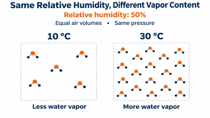
At a fixed relative humidity, warmer conditions generally correspond to more water vapor. A temperature comparison must therefore state whether relative humidity, vapor density, or another moisture quantity remains constant. There is no universal rule that warmer air always causes greater RF attenuation.
Altitude and season change temperature, pressure, and moisture profiles along a route. A prediction should represent those conditions, including their variation with height where relevant. Fencl et al. (2020) found that dry-weather attenuation variations on a 4.86 km E-band link at 73.5 and 83.5 GHz correlated with gaseous attenuation modeled from temperature and humidity observations. They also noted the difficulty of separating gaseous absorption from other propagation losses and equipment effects.
How to Estimate Atmospheric Attenuation Using ITU Models
Select a component model for each relevant loss mechanism and a prediction method suited to the link geometry. The recommendations serve different purposes.
Recommendation | Main use |
Gaseous attenuation | |
Specific rain attenuation | |
Attenuation by liquid-water clouds and fog; stated prediction range 1–200 GHz | |
Terrestrial line-of-sight propagation prediction | |
Earth–space propagation prediction |
For rain, P.838-3 gives:
Here, is rain rate in mm/h and is specific rain attenuation in dB/km. The coefficients and depend on frequency, polarization, and path orientation.
Define the result. Decide whether you need attenuation under stated conditions or a fade level exceeded for a specified percentage of time.
Specify atmospheric inputs. Record frequency, temperature, pressure, and water-vapor density. Follow the model’s pressure convention, distinguishing dry-air pressure from total pressure. Add rain or cloud inputs where required.
Establish path geometry. For Earth–space paths, specify station altitude, elevation angle, and atmospheric profiles. Satellite range includes distance outside the atmosphere; calculate atmospheric loss over the atmospheric portion.
Calculate the relevant components. Apply the selected models and their prescribed path treatment, checking their frequency and geometry limits.
An availability prediction requires atmospheric statistics. Equal-percentile component fades need not occur simultaneously, so adding their individual percentile values does not generally produce the corresponding total fade. Use the applicable method’s prescribed combination rules. When using the combined attenuation from P.618-14, account for its scintillation contribution only once.
Rain Attenuation: From Rain Rate to Path Loss
Rain attenuation along a path depends on the specific attenuation and the length of the path exposed to rain. For a uniform rain rate across a path of length , the path attenuation is:
When rain intensity varies along the path, the total attenuation must account for the local rain conditions over each section. Statistical prediction methods also apply path adjustments because rainfall is rarely uniform across an entire terrestrial or Earth–space link. A measurement at one antenna therefore does not necessarily represent conditions across the whole link. Statistical prediction methods account for this spatial variability through their prescribed path adjustments.
X-Band Atmospheric Attenuation: A Worked 10 GHz Example
A 5 km horizontal link at 10 GHz illustrates how rain can outweigh a small gaseous loss.
Assume one-way propagation at a uniform temperature of 15 °C, total pressure of 1,013.25 hPa, and water-vapor density of 7.5 g/m³. The corresponding dry-air pressure is approximately 1,003.28 hPa.
Compare a gas-only case with 25 mm/h rain covering the entire path, using horizontal polarization. Hold the gaseous conditions unchanged to isolate the added rain loss.
A calculation using ITU-R P.676-13, Annex 1 gives approximately 0.0140 dB/km of gaseous attenuation. For the stated rain case, ITU-R P.838-3, Table 5 gives and , producing approximately 0.696 dB/km of rain attenuation.
Scenario | Gas attenuation (dB/km) | Rain attenuation (dB/km) | Calculated loss over 5 km (dB) |
Gas only | 0.0140 | 0 | 0.070 |
Same gas conditions plus rain | 0.0140 | 0.696 | 3.55 |
For the rain scenario:
Low gaseous absorption therefore does not eliminate the need to evaluate rain loss at X-band. These illustrative results apply to the specified atmosphere and uniform rain extent; they do not establish annual availability.
FAQ
Discussion (0)
Be the first to comment.